I had to go shopping for a family birthday and new apartment stuff this past weekend. I entered the big, bright department store and froze, with instant regret and dread, because I heard the foreboding sounds of this phenomenon:
Now I don’t know about other countries, but in America the tinsel-laden commercial Christmas season stretches starts the day they break down the pop-up Halloween shops and eventually consumes all of popular culture for two months. Hearing Mariah Carey’s “All I Want for Christmas is You” vaguely reminds me of rowing on a river and first hearing the rush of the waters of a gigantic rapid before I see it and it eventually swallows and flips the boat.
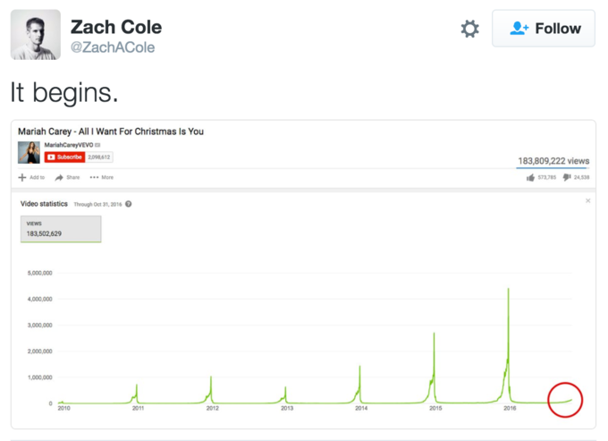
Worried about what the early arrival of the song portended, I sought an
update to Zach Cole’s observation. It turns out that while YouTube’s new layout
hides the “Statistics” button, one can go to the old layout (youtube.com/old/...),
and still find the data. In fact, the raw data is in a hidden table in the page
and is easily grabbed with a little web scrapery:
library(tidyverse)
library(lubridate)
library(stringi)
library(noamtools)
library(broom)
knitr::opts_chunk$set(cache=TRUE)library(RSelenium)
library(rvest)
rD <- rsDriver(browser="phantomjs")
remDr <- rD[["client"]]
remDr$navigate("https://www.youtube.com/old/watch?v=yXQViqx6GMY")
morebutton <- remDr$findElement(using="xpath", '//*[@id="action-panel-overflow-button"]')
morebutton$clickElement()
statsbutton <- remDr$findElement(using="xpath", '//*[@id="action-panel-overflow-menu"]/li[2]/button')
statsbutton$clickElement()
tableelem <- remDr$findElement(using="xpath", '//*[@id="watch-actions-stats"]/div[2]/div[2]/div/div[1]/div/div')
tab <- tableelem$getPageSource()
traffic <- read_html(tab[[1]]) %>%
html_node(xpath = '//*[@id="watch-actions-stats"]/div[2]/div[2]/div/div[1]/div/div/ table') %>%
html_table() %>%
rename(date=Date, views=value) %>%
mutate(date = mdy(date), views = as.numeric(stri_replace_all_fixed(views, ",", "")))
write_csv(mc, "aiwfciy.csv")Sure enough, we are well on our way.
aiwfciy <- read_csv("aiwfciy.csv") %>%
    mutate(date = as.POSIXct(date), yr = year(date), m = month(date), d = day(date), yd = yday(date))

ggplot(aiwfciy, aes(x=date, y=views/1000000, col = (yr == 2017 & m >= 9))) +
    scale_x_datetime() +
    geom_line(size=1) +
    scale_color_manual(values=c("black", "red")) +
    theme_nr +
    scale_y_continuous(breaks=2*(0:4)) +
    theme(axis.title.x=element_blank(), legend.position = "none") +
    labs(y = "Views (millions)", title='Daily YouTube views of Mariah Carey\'s\n"All I Want for Christmas is You"')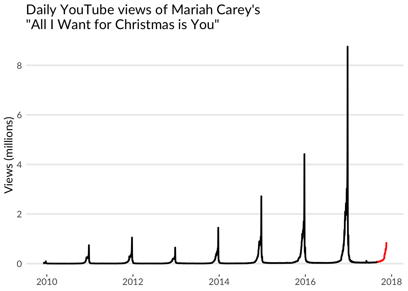
To me, each of these spikes feels like this:

I’m leaving the country for this week, so I’ll be spared a bit of it, but how much will I hear this song in December?
cc <- aiwfciy %>%
    filter(yr !=2009) %>%
    group_by(yr) %>%
    summarize(dec_views = sum(views[m==12]),
              early_nov_views = sum(views[m==11 & d <=15]))

ggplot(filter(cc, yr != 2017), aes(x = as.factor(yr), y=dec_views/1e6)) +
    geom_col() +
    labs(y = "Views (millions)", title='December YouTube views of Mariah Carey\'s\n"All I Want for Christmas is You"') +
    theme_nr +
    theme(axis.title.x=element_blank())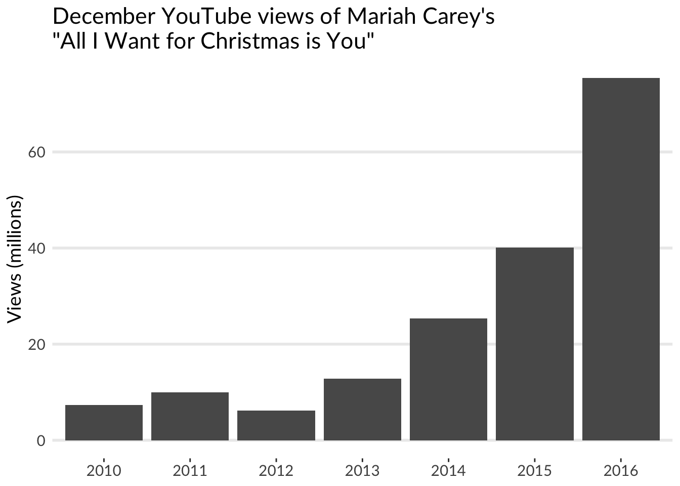
Scarily, views appear to have approximately doubled every year for the past five years. If we fit an exponential growth model like \(\text{XmasCheer}(t) = e^{\lambda t}\), we get this:
expmod <- lm(log(dec_views) ~ yr, data=filter(cc, yr != 2017))
cc <- cc %>%
    mutate(prediction = as.double(exp(predict(expmod, newdata=cc)))) %>%
    mutate(forecast = yr == 2017,
           dec_views = if_else(forecast, prediction, dec_views))

ggplot(cc, aes(x = yr, y=dec_views/1e6)) +
    geom_col(mapping=aes(fill=forecast)) +
    geom_line(mapping=aes(x = yr, y=prediction/1e6), size=1, col="black") +
    geom_point(mapping=aes(x = yr, y=prediction/1e6), size=2, col="black") +
    scale_x_continuous(breaks=2010:2018) +
    scale_y_continuous(breaks = seq(0,100,by=20)) +
    scale_fill_manual(values = c("grey40", "red")) +
    labs(y = "Views (millions)", title='December YouTube views of Mariah Carey\'s\n"All I Want for Christmas is You"') +
    theme_nr +
    theme(axis.title.x=element_blank(), legend.position = "none")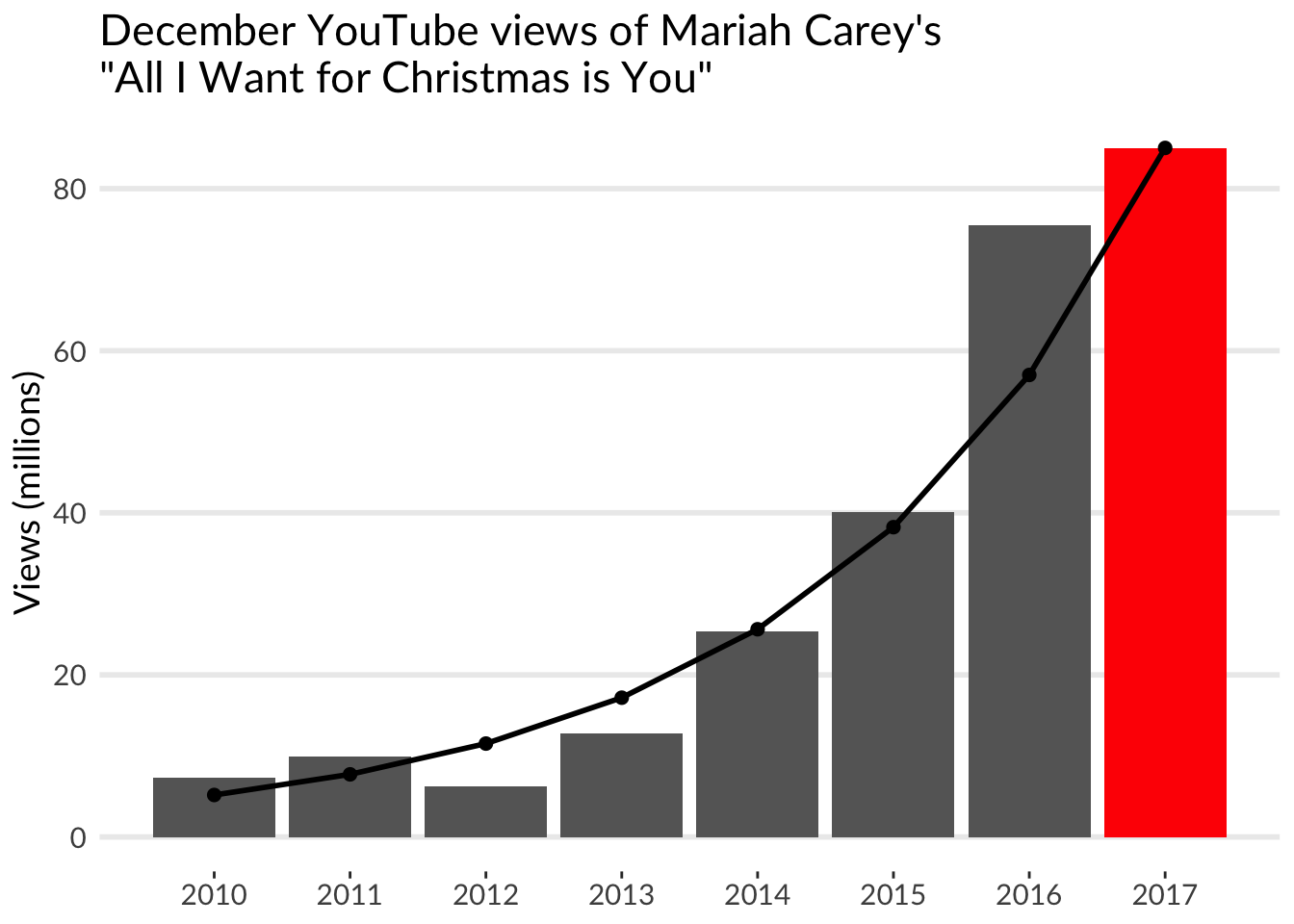
Not bad, though it seems to have underestimated last year’s views by a fair bit, which could actually result in an underestimate this year, too. Based on this model, views will grow ~49% every year and exceed the human population in another 12 years.
As an ecologist, I can thankfully point to a body of theory showing exponential growth is often checked by other mechanisms. For instance, fish consumption of eggs and juveniles limits growth in the Ricker Model, resource limitation can check populations or sometimes environmentally driven stochasticity knocks them back. That is, I can hope this will all collapse into cannibalism, land war or a lucky supervolcano eruption.
Ecologists have a habit of getting things wrong applying ecological models to social processes, though. The Limits to Growth crowd underestimated capitalism’s ability to turn ever more human ingenuity towards its gaping maw. So rather than apply any of these mechanisms, let’s take a one-step-ahead approach and see what last weekend’s shopping experience tells us about what’s to come.
It turns out there is a very good correlation between views in the first two weeks of November and the size of the beast in December:
lmod <- lm(log10(dec_views) ~ log10(early_nov_views), data = filter(cc, yr != 2017))
summary(lmod)
##
## Call:
## lm(formula = log10(dec_views) ~ log10(early_nov_views), data = filter(cc,
## yr != 2017))
##
## Residuals:
## 1 2 3 4 5 6 7
## 0.09642 -0.01987 -0.12575 0.03236 0.01967 -0.02068 0.01785
##
## Coefficients:
## Estimate Std. Error t value Pr(>|t|)
## (Intercept) 1.49562 0.44020 3.398 0.0193 *
## log10(early_nov_views) 0.94195 0.07199 13.085 4.65e-05 ***
## ---
## Signif. codes: 0 '***' 0.001 '**' 0.01 '*' 0.05 '.' 0.1 ' ' 1
##
## Residual standard error: 0.07441 on 5 degrees of freedom
## Multiple R-squared: 0.9716, Adjusted R-squared: 0.966
## F-statistic: 171.2 on 1 and 5 DF, p-value: 4.652e-05ggplot(filter(cc, yr != 2017), aes(x = log10(early_nov_views), y = log10(dec_views))) +
geom_smooth(method=lm) +
geom_point() +
theme_nr + theme(panel.grid.major.x = element_line(color="grey10", size=0.5),
panel.grid.major.y = element_line(color="grey10", size=0.25)) +
labs(title = "Correlation Between WAY EARLY November views\nand just excessive December views",
x = "log10(Total views in the first half of November)",
y = "log10(Total views in December)")## `geom_smooth()` using formula 'y ~ x'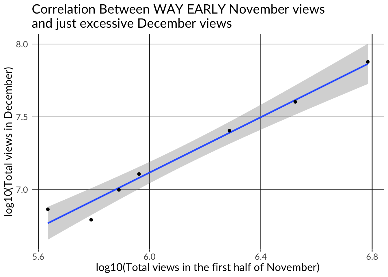
With this, we can make an alternative projection:
cc <- cc %>%
    mutate(pred2 = as.double(10^predict(lmod, newdata=cc)),
           dec_views = if_else(forecast, pred2, dec_views))

ggplot(cc, aes(x = yr, y=dec_views/1e6)) +
    geom_col(mapping=aes(fill=forecast)) +
    geom_line(mapping=aes(x = yr, y=pred2/1e6), size=1, col="black") +
    geom_point(mapping=aes(x = yr, y=pred2/1e6), size=2, col="black") +
    scale_x_continuous(breaks=2010:2018) +
    scale_y_continuous(breaks = seq(0,100,by=20)) +
    labs(y = "Views (millions)", title='December YouTube views of Mariah Carey\'s\n"All I Want for Christmas is You"') +
    scale_fill_manual(values = c("grey40", "red")) +
    theme_nr +
    theme(axis.title.x=element_blank(), legend.position = "none")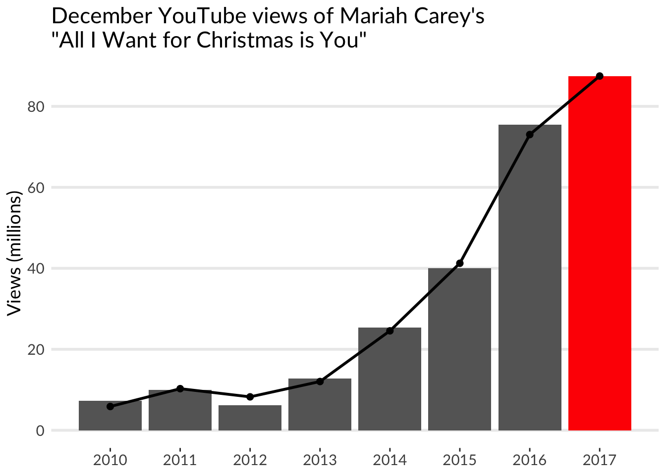
We get almost the same result! Though maybe, just maybe, the flood has lost some momentum this year.
Happy Holidays.