Today at Davis R Users’ Group, Rosemary Hartman took us through her work in progress fitting general additive models to organism presence/absence data. Below is her presentation and script. You can get the original script and data here
Also, check the comments below for some discussion of other options for this type of analysis, such as boosted regression trees.
## GAMs using mgcv and amphibian presence/absence dataset
## code and data by Rosemary Hartman (rosehartman at gmail dot com)
## First, load the mgcv package (Simon Wood)
library(mgcv)
## Now, attach your data set (or my data set)
fishlakes <- read.csv("fishlakes.csv", comment.char="#")
## create a full exploritory model using varibles you think are biologically
## significant (this is pretty subjective, and where you need to use your brain)
## For my data set, I am trying to predict the presence of cascades frogs
fishlakes.logr <- gam(treatment ~ ## "treatment" = breeding cascades frogs in lake
BUBO.breeding + ## breeding toads in lake
count.RACApops.1K + ## number of cascades frog populations within 1km
s(silt.total, k=6) + ## amount of silt in lake bed
s(vegetated.area, k=7) + ## total lake area with emergent aquatic vegetation
s(area.10cm, k=6) + ## total lake area less than 10cm deep
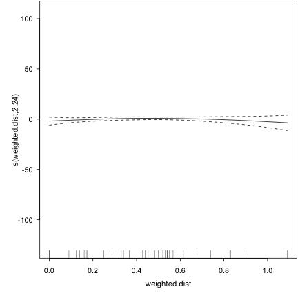
s(weighted.dist, k=6) + ## perportion of nearby water bodies with frogs weighted by distance
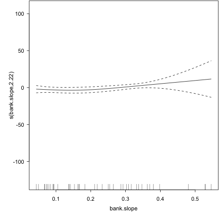
s(bank.slope, k=6), ## average slope
family=binomial("logit"), data= fishlakes) ## this is a logistic function since I have binomial data## Warning: matrix not positive definite##
## Family: binomial
## Link function: logit
##
## Formula:
## treatment ~ BUBO.breeding + count.RACApops.1K + s(silt.total,
## k = 6) + s(vegetated.area, k = 7) + s(area.10cm, k = 6) +
## s(weighted.dist, k = 6) + s(bank.slope, k = 6)
##
## Parametric coefficients:
## Estimate Std. Error z value Pr(>|z|)
## (Intercept) 3.830 3.224 1.19 0.235
## BUBO.breedingy -3.393 1.646 -2.06 0.039 *
## count.RACApops.1K -0.192 0.506 -0.38 0.705
## ---
## Signif. codes: 0 '***' 0.001 '**' 0.01 '*' 0.05 '.' 0.1 ' ' 1
##
## Approximate significance of smooth terms:
## edf Ref.df Chi.sq p-value
## s(silt.total) 1.00 1.00 0.51 0.47
## s(vegetated.area) 3.48 3.97 3.47 0.48
## s(area.10cm) 2.20 2.66 1.17 0.70
## s(weighted.dist) 2.24 2.73 2.56 0.41
## s(bank.slope) 2.22 2.68 5.02 0.14
##
## R-sq.(adj) = 0.597 Deviance explained = 68.5%
## UBRE score = 0.091416 Scale est. = 1 n = 42##
## Method: UBRE Optimizer: outer newton
## full convergence after 14 iterations.
## Gradient range [-4.272e-07,2.326e-07]
## (score 0.09142 & scale 1).
## Hessian positive definite, eigenvalue range [2.564e-07,0.05689].
##
## Basis dimension (k) checking results. Low p-value (k-index<1) may
## indicate that k is too low, especially if edf is close to k'.
##
## k' edf k-index p-value
## s(silt.total) 5.000 1.000 0.691 0.02
## s(vegetated.area) 6.000 3.485 1.321 0.97
## s(area.10cm) 5.000 2.200 0.742 0.02
## s(weighted.dist) 5.000 2.237 1.064 0.63
## s(bank.slope) 5.000 2.219 0.965 0.42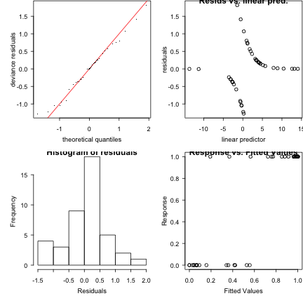
## gives huge overspecification. I'm not sure what to do about this.
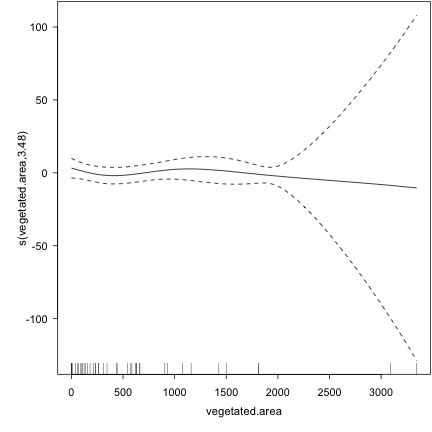
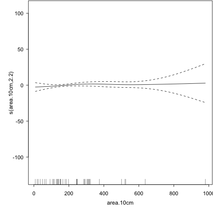
plot(fishlakes.logr) ## diagnostic plots for the smooths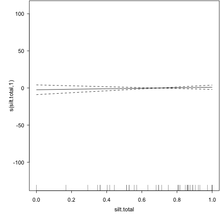
## To choose my k's, I looped through a bunch of different values for k, and basically
## just played around until my model stopped overspecifying


for (i in 2:8) { fishlakes.logr <- gam(treatment ~ count.RACApops.1K + BUBO.breeding + s(silt.total, k=i) + s(vegetated.area, k=i) + s(bank.slope, k=i) + s(area.10cm,  k=i) + s(weighted.dist, k=i), family=binomial("logit"), data= fishlakes);
                  x <- summary(fishlakes.logr);
                  y <- AIC(fishlakes.logr);
                  print(i)
                  print(x)
                  print(y)
}
## Warning: basis dimension, k, increased to minimum possible
## Warning: basis dimension, k, increased to minimum possible
## Warning: basis dimension, k, increased to minimum possible
## Warning: basis dimension, k, increased to minimum possible
## Warning: basis dimension, k, increased to minimum possible
## Warning: matrix not positive definite
## Warning: matrix not positive definite
## Warning: matrix not positive definite
## Warning: matrix not positive definite
## [1] 2
##
## Family: binomial
## Link function: logit
##
## Formula:
## treatment ~ count.RACApops.1K + BUBO.breeding + s(silt.total,
## k = i) + s(vegetated.area, k = i) + s(bank.slope, k = i) +
## s(area.10cm, k = i) + s(weighted.dist, k = i)
##
## Parametric coefficients:
## Estimate Std. Error z value Pr(>|z|)
## (Intercept) 3.011 1.263 2.38 0.017 *
## count.RACApops.1K -0.247 0.307 -0.80 0.421
## BUBO.breedingy -2.314 1.010 -2.29 0.022 *
## ---
## Signif. codes: 0 '***' 0.001 '**' 0.01 '*' 0.05 '.' 0.1 ' ' 1
##
## Approximate significance of smooth terms:
## edf Ref.df Chi.sq p-value
## s(silt.total) 1.00 1.00 0.05 0.82
## s(vegetated.area) 1.00 1.00 0.27 0.61
## s(bank.slope) 1.63 1.86 1.97 0.34
## s(area.10cm) 1.00 1.00 0.04 0.85
## s(weighted.dist) 1.80 1.96 2.34 0.30
##
## R-sq.(adj) = 0.339 Deviance explained = 42.2%
## UBRE score = 0.21726 Scale est. = 1 n = 42
## [1] 51.12
## Warning: matrix not positive definite
## Warning: matrix not positive definite
## Warning: matrix not positive definite
## Warning: matrix not positive definite
## [1] 3
##
## Family: binomial
## Link function: logit
##
## Formula:
## treatment ~ count.RACApops.1K + BUBO.breeding + s(silt.total,
## k = i) + s(vegetated.area, k = i) + s(bank.slope, k = i) +
## s(area.10cm, k = i) + s(weighted.dist, k = i)
##
## Parametric coefficients:
## Estimate Std. Error z value Pr(>|z|)
## (Intercept) 3.011 1.263 2.38 0.017 *
## count.RACApops.1K -0.247 0.307 -0.80 0.421
## BUBO.breedingy -2.314 1.010 -2.29 0.022 *
## ---
## Signif. codes: 0 '***' 0.001 '**' 0.01 '*' 0.05 '.' 0.1 ' ' 1
##
## Approximate significance of smooth terms:
## edf Ref.df Chi.sq p-value
## s(silt.total) 1.00 1.00 0.05 0.82
## s(vegetated.area) 1.00 1.00 0.27 0.61
## s(bank.slope) 1.63 1.86 1.97 0.34
## s(area.10cm) 1.00 1.00 0.04 0.85
## s(weighted.dist) 1.80 1.96 2.34 0.30
##
## R-sq.(adj) = 0.339 Deviance explained = 42.2%
## UBRE score = 0.21726 Scale est. = 1 n = 42
## [1] 51.12
## Warning: matrix not positive definite
## Warning: matrix not positive definite
## Warning: matrix not positive definite
## Warning: matrix not positive definite
## [1] 4
##
## Family: binomial
## Link function: logit
##
## Formula:
## treatment ~ count.RACApops.1K + BUBO.breeding + s(silt.total,
## k = i) + s(vegetated.area, k = i) + s(bank.slope, k = i) +
## s(area.10cm, k = i) + s(weighted.dist, k = i)
##
## Parametric coefficients:
## Estimate Std. Error z value Pr(>|z|)
## (Intercept) 2.745 1.147 2.39 0.017 *
## count.RACApops.1K -0.217 0.299 -0.73 0.468
## BUBO.breedingy -2.308 0.996 -2.32 0.020 *
## ---
## Signif. codes: 0 '***' 0.001 '**' 0.01 '*' 0.05 '.' 0.1 ' ' 1
##
## Approximate significance of smooth terms:
## edf Ref.df Chi.sq p-value
## s(silt.total) 1.00 1.00 0.06 0.81
## s(vegetated.area) 1.00 1.00 0.31 0.58
## s(bank.slope) 1.77 2.14 2.38 0.33
## s(area.10cm) 1.00 1.00 0.08 0.78
## s(weighted.dist) 1.86 2.25 2.53 0.32
##
## R-sq.(adj) = 0.332 Deviance explained = 42%
## UBRE score = 0.22873 Scale est. = 1 n = 42
## [1] 51.61
## Warning: matrix not positive definite
## Warning: matrix not positive definite
## Warning: matrix not positive definite
## [1] 5
##
## Family: binomial
## Link function: logit
##
## Formula:
## treatment ~ count.RACApops.1K + BUBO.breeding + s(silt.total,
## k = i) + s(vegetated.area, k = i) + s(bank.slope, k = i) +
## s(area.10cm, k = i) + s(weighted.dist, k = i)
##
## Parametric coefficients:
## Estimate Std. Error z value Pr(>|z|)
## (Intercept) -16.5 4857.1 0.00 1.00
## count.RACApops.1K 42.4 397.8 0.11 0.92
## BUBO.breedingy -254.6 9152.1 -0.03 0.98
##
## Approximate significance of smooth terms:
## edf Ref.df Chi.sq p-value
## s(silt.total) 1.00 1.00 0.00 0.95
## s(vegetated.area) 2.32 2.36 0.00 1.00
## s(bank.slope) 1.52 1.57 0.01 0.99
## s(area.10cm) 3.06 3.07 0.02 1.00
## s(weighted.dist) 4.00 4.00 0.02 1.00
##
## R-sq.(adj) = 1 Deviance explained = 100%
## UBRE score = -0.29037 Scale est. = 1 n = 42
## [1] 29.8
## Warning: matrix not positive definite
## [1] 6
##
## Family: binomial
## Link function: logit
##
## Formula:
## treatment ~ count.RACApops.1K + BUBO.breeding + s(silt.total,
## k = i) + s(vegetated.area, k = i) + s(bank.slope, k = i) +
## s(area.10cm, k = i) + s(weighted.dist, k = i)
##
## Parametric coefficients:
## Estimate Std. Error z value Pr(>|z|)
## (Intercept) 5.4778 2.5608 2.14 0.032 *
## count.RACApops.1K -0.0673 0.4763 -0.14 0.888
## BUBO.breedingy -4.9379 2.1801 -2.26 0.024 *
## ---
## Signif. codes: 0 '***' 0.001 '**' 0.01 '*' 0.05 '.' 0.1 ' ' 1
##
## Approximate significance of smooth terms:
## edf Ref.df Chi.sq p-value
## s(silt.total) 1.00 1.00 0.14 0.71
## s(vegetated.area) 1.00 1.00 0.38 0.54
## s(bank.slope) 2.14 2.60 3.51 0.25
## s(area.10cm) 5.00 5.00 5.46 0.36
## s(weighted.dist) 2.13 2.64 2.50 0.40
##
## R-sq.(adj) = 0.523 Deviance explained = 65.4%
## UBRE score = 0.13954 Scale est. = 1 n = 42
## [1] 47.86
## [1] 7
##
## Family: binomial
## Link function: logit
##
## Formula:
## treatment ~ count.RACApops.1K + BUBO.breeding + s(silt.total,
## k = i) + s(vegetated.area, k = i) + s(bank.slope, k = i) +
## s(area.10cm, k = i) + s(weighted.dist, k = i)
##
## Parametric coefficients:
## Estimate Std. Error z value Pr(>|z|)
## (Intercept) 6.56 366.37 0.02 0.99
## count.RACApops.1K 4.30 13.89 0.31 0.76
## BUBO.breedingy -22.94 36.65 -0.63 0.53
##
## Approximate significance of smooth terms:
## edf Ref.df Chi.sq p-value
## s(silt.total) 1.00 1.00 0.02 0.88
## s(vegetated.area) 3.50 3.82 0.97 0.90
## s(bank.slope) 1.00 1.00 0.13 0.72
## s(area.10cm) 1.00 1.00 0.61 0.44
## s(weighted.dist) 4.02 4.21 1.32 0.88
##
## R-sq.(adj) = 1 Deviance explained = 99.7%
## UBRE score = -0.35283 Scale est. = 1 n = 42
## [1] 27.18
## Warning: matrix not positive definite
## Warning: matrix not positive definite
## Warning: matrix not positive definite
## Warning: matrix not positive definite
## [1] 8
##
## Family: binomial
## Link function: logit
##
## Formula:
## treatment ~ count.RACApops.1K + BUBO.breeding + s(silt.total,
## k = i) + s(vegetated.area, k = i) + s(bank.slope, k = i) +
## s(area.10cm, k = i) + s(weighted.dist, k = i)
##
## Parametric coefficients:
## Estimate Std. Error z value Pr(>|z|)
## (Intercept) 22.752 135.686 0.17 0.87
## count.RACApops.1K -0.247 23.133 -0.01 0.99
## BUBO.breedingy -29.877 67.934 -0.44 0.66
##
## Approximate significance of smooth terms:
## edf Ref.df Chi.sq p-value
## s(silt.total) 4.58 4.71 0.09 1.00
## s(vegetated.area) 3.19 3.31 0.01 1.00
## s(bank.slope) 1.00 1.00 0.06 0.80
## s(area.10cm) 2.14 2.23 0.02 0.99
## s(weighted.dist) 3.68 3.87 0.04 1.00
##
## R-sq.(adj) = 1 Deviance explained = 99.9%
## UBRE score = -0.16157 Scale est. = 1 n = 42
## [1] 35.21
for (i in 2:10) { fishlakes.logr <- gam(treatment ~ count.RACApops.1K + BUBO.breeding + s(silt.total, k=i) + s(vegetated.area, k=7) + s(bank.slope, k=6) + s(area.10cm,  k=6) + s(weighted.dist, k=6), family=binomial("logit"), data= fishlakes);
                  x <- summary(fishlakes.logr);
                  y <- AIC(fishlakes.logr);
                  print(i)
                  print(x)
                  print(y)
}
## Warning: basis dimension, k, increased to minimum possible
## Warning: matrix not positive definite
## [1] 2
##
## Family: binomial
## Link function: logit
##
## Formula:
## treatment ~ count.RACApops.1K + BUBO.breeding + s(silt.total,
## k = i) + s(vegetated.area, k = 7) + s(bank.slope, k = 6) +
## s(area.10cm, k = 6) + s(weighted.dist, k = 6)
##
## Parametric coefficients:
## Estimate Std. Error z value Pr(>|z|)
## (Intercept) 5.4778 2.5608 2.14 0.032 *
## count.RACApops.1K -0.0673 0.4763 -0.14 0.888
## BUBO.breedingy -4.9379 2.1801 -2.26 0.024 *
## ---
## Signif. codes: 0 '***' 0.001 '**' 0.01 '*' 0.05 '.' 0.1 ' ' 1
##
## Approximate significance of smooth terms:
## edf Ref.df Chi.sq p-value
## s(silt.total) 1.00 1.00 0.14 0.71
## s(vegetated.area) 1.00 1.00 0.38 0.54
## s(bank.slope) 2.14 2.60 3.51 0.25
## s(area.10cm) 5.00 5.00 5.46 0.36
## s(weighted.dist) 2.13 2.64 2.50 0.40
##
## R-sq.(adj) = 0.523 Deviance explained = 65.4%
## UBRE score = 0.13954 Scale est. = 1 n = 42
## [1] 47.86
## Warning: matrix not positive definite
## [1] 3
##
## Family: binomial
## Link function: logit
##
## Formula:
## treatment ~ count.RACApops.1K + BUBO.breeding + s(silt.total,
## k = i) + s(vegetated.area, k = 7) + s(bank.slope, k = 6) +
## s(area.10cm, k = 6) + s(weighted.dist, k = 6)
##
## Parametric coefficients:
## Estimate Std. Error z value Pr(>|z|)
## (Intercept) 5.4778 2.5608 2.14 0.032 *
## count.RACApops.1K -0.0673 0.4763 -0.14 0.888
## BUBO.breedingy -4.9379 2.1801 -2.26 0.024 *
## ---
## Signif. codes: 0 '***' 0.001 '**' 0.01 '*' 0.05 '.' 0.1 ' ' 1
##
## Approximate significance of smooth terms:
## edf Ref.df Chi.sq p-value
## s(silt.total) 1.00 1.00 0.14 0.71
## s(vegetated.area) 1.00 1.00 0.38 0.54
## s(bank.slope) 2.14 2.60 3.51 0.25
## s(area.10cm) 5.00 5.00 5.46 0.36
## s(weighted.dist) 2.13 2.64 2.50 0.40
##
## R-sq.(adj) = 0.523 Deviance explained = 65.4%
## UBRE score = 0.13954 Scale est. = 1 n = 42
## [1] 47.86
## [1] 4
##
## Family: binomial
## Link function: logit
##
## Formula:
## treatment ~ count.RACApops.1K + BUBO.breeding + s(silt.total,
## k = i) + s(vegetated.area, k = 7) + s(bank.slope, k = 6) +
## s(area.10cm, k = 6) + s(weighted.dist, k = 6)
##
## Parametric coefficients:
## Estimate Std. Error z value Pr(>|z|)
## (Intercept) 76.6 427.3 0.18 0.86
## count.RACApops.1K 10.1 51.7 0.20 0.84
## BUBO.breedingy -89.3 536.3 -0.17 0.87
##
## Approximate significance of smooth terms:
## edf Ref.df Chi.sq p-value
## s(silt.total) 1.00 1.00 0.00 0.97
## s(vegetated.area) 2.65 2.70 0.03 1.00
## s(bank.slope) 3.77 3.87 0.12 1.00
## s(area.10cm) 4.51 4.54 0.19 1.00
## s(weighted.dist) 1.87 1.90 0.03 0.98
##
## R-sq.(adj) = 1 Deviance explained = 100%
## UBRE score = -0.19934 Scale est. = 1 n = 42
## [1] 33.63
## Warning: matrix not positive definite
## [1] 5
##
## Family: binomial
## Link function: logit
##
## Formula:
## treatment ~ count.RACApops.1K + BUBO.breeding + s(silt.total,
## k = i) + s(vegetated.area, k = 7) + s(bank.slope, k = 6) +
## s(area.10cm, k = 6) + s(weighted.dist, k = 6)
##
## Parametric coefficients:
## Estimate Std. Error z value Pr(>|z|)
## (Intercept) 5.4778 2.5609 2.14 0.032 *
## count.RACApops.1K -0.0673 0.4763 -0.14 0.888
## BUBO.breedingy -4.9379 2.1801 -2.26 0.024 *
## ---
## Signif. codes: 0 '***' 0.001 '**' 0.01 '*' 0.05 '.' 0.1 ' ' 1
##
## Approximate significance of smooth terms:
## edf Ref.df Chi.sq p-value
## s(silt.total) 1.00 1.00 0.14 0.71
## s(vegetated.area) 1.00 1.00 0.38 0.54
## s(bank.slope) 2.14 2.60 3.51 0.25
## s(area.10cm) 5.00 5.00 5.46 0.36
## s(weighted.dist) 2.13 2.64 2.50 0.40
##
## R-sq.(adj) = 0.523 Deviance explained = 65.4%
## UBRE score = 0.13954 Scale est. = 1 n = 42
## [1] 47.86
## Warning: matrix not positive definite
## [1] 6
##
## Family: binomial
## Link function: logit
##
## Formula:
## treatment ~ count.RACApops.1K + BUBO.breeding + s(silt.total,
## k = i) + s(vegetated.area, k = 7) + s(bank.slope, k = 6) +
## s(area.10cm, k = 6) + s(weighted.dist, k = 6)
##
## Parametric coefficients:
## Estimate Std. Error z value Pr(>|z|)
## (Intercept) 3.830 3.224 1.19 0.235
## count.RACApops.1K -0.192 0.506 -0.38 0.705
## BUBO.breedingy -3.393 1.646 -2.06 0.039 *
## ---
## Signif. codes: 0 '***' 0.001 '**' 0.01 '*' 0.05 '.' 0.1 ' ' 1
##
## Approximate significance of smooth terms:
## edf Ref.df Chi.sq p-value
## s(silt.total) 1.00 1.00 0.51 0.47
## s(vegetated.area) 3.48 3.97 3.47 0.48
## s(bank.slope) 2.22 2.68 4.07 0.21
## s(area.10cm) 2.20 2.66 1.09 0.72
## s(weighted.dist) 2.24 2.73 1.90 0.54
##
## R-sq.(adj) = 0.597 Deviance explained = 68.5%
## UBRE score = 0.091416 Scale est. = 1 n = 42
## [1] 45.84
## [1] 7
##
## Family: binomial
## Link function: logit
##
## Formula:
## treatment ~ count.RACApops.1K + BUBO.breeding + s(silt.total,
## k = i) + s(vegetated.area, k = 7) + s(bank.slope, k = 6) +
## s(area.10cm, k = 6) + s(weighted.dist, k = 6)
##
## Parametric coefficients:
## Estimate Std. Error z value Pr(>|z|)
## (Intercept) 55.26 358.87 0.15 0.88
## count.RACApops.1K 5.42 99.67 0.05 0.96
## BUBO.breedingy -87.21 624.65 -0.14 0.89
##
## Approximate significance of smooth terms:
## edf Ref.df Chi.sq p-value
## s(silt.total) 4.96 4.99 0.09 1.00
## s(vegetated.area) 3.99 4.02 0.02 1.00
## s(bank.slope) 1.00 1.00 0.01 0.93
## s(area.10cm) 1.86 1.96 0.02 0.99
## s(weighted.dist) 1.03 1.03 0.01 0.92
##
## R-sq.(adj) = 1 Deviance explained = 100%
## UBRE score = -0.24525 Scale est. = 1 n = 42
## [1] 31.7
## Warning: matrix not positive definite
## [1] 8
##
## Family: binomial
## Link function: logit
##
## Formula:
## treatment ~ count.RACApops.1K + BUBO.breeding + s(silt.total,
## k = i) + s(vegetated.area, k = 7) + s(bank.slope, k = 6) +
## s(area.10cm, k = 6) + s(weighted.dist, k = 6)
##
## Parametric coefficients:
## Estimate Std. Error z value Pr(>|z|)
## (Intercept) 89.75 12140.84 0.01 0.99
## count.RACApops.1K -3.53 1710.88 0.00 1.00
## BUBO.breedingy -119.62 9443.72 -0.01 0.99
##
## Approximate significance of smooth terms:
## edf Ref.df Chi.sq p-value
## s(silt.total) 5.76 5.80 0 1
## s(vegetated.area) 2.03 2.04 0 1
## s(bank.slope) 1.18 1.19 0 1
## s(area.10cm) 1.84 1.90 0 1
## s(weighted.dist) 1.08 1.08 0 1
##
## R-sq.(adj) = 1 Deviance explained = 100%
## UBRE score = -0.29122 Scale est. = 1 n = 42
## [1] 29.77
## [1] 9
##
## Family: binomial
## Link function: logit
##
## Formula:
## treatment ~ count.RACApops.1K + BUBO.breeding + s(silt.total,
## k = i) + s(vegetated.area, k = 7) + s(bank.slope, k = 6) +
## s(area.10cm, k = 6) + s(weighted.dist, k = 6)
##
## Parametric coefficients:
## Estimate Std. Error z value Pr(>|z|)
## (Intercept) 48.947 655.719 0.07 0.94
## count.RACApops.1K -0.137 82.969 0.00 1.00
## BUBO.breedingy -73.934 546.328 -0.14 0.89
##
## Approximate significance of smooth terms:
## edf Ref.df Chi.sq p-value
## s(silt.total) 5.75 5.84 0.02 1.00
## s(vegetated.area) 2.00 2.01 0.01 1.00
## s(bank.slope) 1.00 1.00 0.01 0.91
## s(area.10cm) 1.86 1.95 0.01 0.99
## s(weighted.dist) 1.19 1.21 0.00 0.99
##
## R-sq.(adj) = 1 Deviance explained = 100%
## UBRE score = -0.29492 Scale est. = 1 n = 42
## [1] 29.61
## [1] 10
##
## Family: binomial
## Link function: logit
##
## Formula:
## treatment ~ count.RACApops.1K + BUBO.breeding + s(silt.total,
## k = i) + s(vegetated.area, k = 7) + s(bank.slope, k = 6) +
## s(area.10cm, k = 6) + s(weighted.dist, k = 6)
##
## Parametric coefficients:
## Estimate Std. Error z value Pr(>|z|)
## (Intercept) 54.2952 102.0865 0.53 0.59
## count.RACApops.1K -0.0411 16.5558 0.00 1.00
## BUBO.breedingy -75.4705 126.5539 -0.60 0.55
##
## Approximate significance of smooth terms:
## edf Ref.df Chi.sq p-value
## s(silt.total) 6.88 7.06 0.74 1.00
## s(vegetated.area) 3.09 3.16 0.22 0.98
## s(bank.slope) 1.04 1.05 0.22 0.66
## s(area.10cm) 2.42 2.67 0.38 0.92
## s(weighted.dist) 1.00 1.00 0.30 0.58
##
## R-sq.(adj) = 1 Deviance explained = 99.8%
## UBRE score = -0.16704 Scale est. = 1 n = 42
## [1] 34.98
## In order to see which of the candidate terms are significant, I will run the model
## several times, dropping one term out each time and then do a likelyhood ratio test
## to see if adding the term leads to a significant improvement in residual deviance.

## fishlakes2.logr is the same model as fishlakes.logr without the "bank slope" term
fishlakes2.logr <- gam(treatment ~ BUBO.breeding + count.RACApops.1K +
  s(silt.total, k=6) + s(vegetated.area, k=7) + s(area.10cm, k=6) + s(weighted.dist, k=6),
                       family=binomial("logit"), data= fishlakes)
## Warning: matrix not positive definite##
## Family: binomial
## Link function: logit
##
## Formula:
## treatment ~ BUBO.breeding + count.RACApops.1K + s(silt.total,
## k = 6) + s(vegetated.area, k = 7) + s(area.10cm, k = 6) +
## s(weighted.dist, k = 6)
##
## Parametric coefficients:
## Estimate Std. Error z value Pr(>|z|)
## (Intercept) 2.175 0.974 2.23 0.026 *
## BUBO.breedingy -1.840 0.891 -2.07 0.039 *
## count.RACApops.1K -0.294 0.290 -1.01 0.311
## ---
## Signif. codes: 0 '***' 0.001 '**' 0.01 '*' 0.05 '.' 0.1 ' ' 1
##
## Approximate significance of smooth terms:
## edf Ref.df Chi.sq p-value
## s(silt.total) 1.00 1.00 3.19 0.074 .
## s(vegetated.area) 1.00 1.00 0.46 0.499
## s(area.10cm) 1.00 1.00 1.82 0.177
## s(weighted.dist) 2.02 2.54 2.53 0.375
## ---
## Signif. codes: 0 '***' 0.001 '**' 0.01 '*' 0.05 '.' 0.1 ' ' 1
##
## R-sq.(adj) = 0.279 Deviance explained = 34.1%
## UBRE score = 0.25725 Scale est. = 1 n = 42## Analysis of Deviance Table
##
## Model 1: treatment ~ BUBO.breeding + count.RACApops.1K + s(silt.total,
## k = 6) + s(vegetated.area, k = 7) + s(area.10cm, k = 6) +
## s(weighted.dist, k = 6)
## Model 2: treatment ~ count.RACApops.1K + BUBO.breeding + s(silt.total,
## k = i) + s(vegetated.area, k = 7) + s(bank.slope, k = 6) +
## s(area.10cm, k = 6) + s(weighted.dist, k = 6)
## Resid. Df Resid. Dev Df Deviance Pr(>Chi)
## 1 34.0 36.8
## 2 24.6 0.1 9.41 36.6 4.2e-05 ***
## ---
## Signif. codes: 0 '***' 0.001 '**' 0.01 '*' 0.05 '.' 0.1 ' ' 1 ## in explanitory power between the two models, that means the "bank slope" term
## should be included in the final model
## Now do the same with the rest of the varibles
fishlakes3.logr <- gam(treatment ~ BUBO.breeding + count.RACApops.1K +s(silt.total, k=6)
+ s(vegetated.area, k=7) + s(bank.slope, k=6) + s(area.10cm, k=6),
family=binomial("logit"), data= fishlakes) ## all variables except "weighted distance"## Warning: matrix not positive definite##
## Family: binomial
## Link function: logit
##
## Formula:
## treatment ~ BUBO.breeding + count.RACApops.1K + s(silt.total,
## k = 6) + s(vegetated.area, k = 7) + s(bank.slope, k = 6) +
## s(area.10cm, k = 6)
##
## Parametric coefficients:
## Estimate Std. Error z value Pr(>|z|)
## (Intercept) 77.43 282.28 0.27 0.78
## BUBO.breedingy -120.75 510.54 -0.24 0.81
## count.RACApops.1K 2.83 64.25 0.04 0.96
##
## Approximate significance of smooth terms:
## edf Ref.df Chi.sq p-value
## s(silt.total) 4.77 4.80 0.08 1.00
## s(vegetated.area) 2.15 2.19 0.02 0.99
## s(bank.slope) 1.22 1.25 0.06 0.88
## s(area.10cm) 3.71 3.77 0.06 1.00
##
## R-sq.(adj) = 1 Deviance explained = 100%
## UBRE score = -0.29299 Scale est. = 1 n = 42## Analysis of Deviance Table
##
## Model 1: treatment ~ BUBO.breeding + count.RACApops.1K + s(silt.total,
## k = 6) + s(vegetated.area, k = 7) + s(bank.slope, k = 6) +
## s(area.10cm, k = 6)
## Model 2: treatment ~ count.RACApops.1K + BUBO.breeding + s(silt.total,
## k = i) + s(vegetated.area, k = 7) + s(bank.slope, k = 6) +
## s(area.10cm, k = 6) + s(weighted.dist, k = 6)
## Resid. Df Resid. Dev Df Deviance Pr(>Chi)
## 1 27.2 0.008
## 2 24.6 0.127 2.59 -0.119 ## Include "weighted distance" in final model
fishlakes4.logr <- gam(treatment ~ BUBO.breeding +count.RACApops.1K+
s(silt.total, k=6) + s(vegetated.area, k=7) +
s(bank.slope, k=6) + s(weighted.dist, k=6),
family=binomial("logit"), data= fishlakes) ## all variables except area under 10cm## Warning: matrix not positive definite##
## Family: binomial
## Link function: logit
##
## Formula:
## treatment ~ BUBO.breeding + count.RACApops.1K + s(silt.total,
## k = 6) + s(vegetated.area, k = 7) + s(bank.slope, k = 6) +
## s(weighted.dist, k = 6)
##
## Parametric coefficients:
## Estimate Std. Error z value Pr(>|z|)
## (Intercept) 2.490 1.851 1.35 0.179
## BUBO.breedingy -1.997 1.100 -1.82 0.069 .
## count.RACApops.1K -0.465 0.373 -1.25 0.213
## ---
## Signif. codes: 0 '***' 0.001 '**' 0.01 '*' 0.05 '.' 0.1 ' ' 1
##
## Approximate significance of smooth terms:
## edf Ref.df Chi.sq p-value
## s(silt.total) 1.00 1.00 0.03 0.852
## s(vegetated.area) 3.29 3.81 4.86 0.276
## s(bank.slope) 1.00 1.00 4.12 0.042 *
## s(weighted.dist) 1.40 1.70 0.81 0.591
## ---
## Signif. codes: 0 '***' 0.001 '**' 0.01 '*' 0.05 '.' 0.1 ' ' 1
##
## R-sq.(adj) = 0.513 Deviance explained = 54.5%
## UBRE score = 0.066475 Scale est. = 1 n = 42## Analysis of Deviance Table
##
## Model 1: treatment ~ BUBO.breeding + count.RACApops.1K + s(silt.total,
## k = 6) + s(vegetated.area, k = 7) + s(bank.slope, k = 6) +
## s(weighted.dist, k = 6)
## Model 2: treatment ~ count.RACApops.1K + BUBO.breeding + s(silt.total,
## k = i) + s(vegetated.area, k = 7) + s(bank.slope, k = 6) +
## s(area.10cm, k = 6) + s(weighted.dist, k = 6)
## Resid. Df Resid. Dev Df Deviance Pr(>Chi)
## 1 32.3 25.40
## 2 24.6 0.13 7.73 25.3 0.0012 **
## ---
## Signif. codes: 0 '***' 0.001 '**' 0.01 '*' 0.05 '.' 0.1 ' ' 1 ## significant, leave "area under 10cm" out of final model
fishlakes5.logr <- gam(treatment ~ BUBO.breeding +
s(silt.total, k=6) + s(vegetated.area, k=7)+ s(area.10cm, k=6) +
s(weighted.dist, k=6), family=binomial("logit"), data= fishlakes) ## all variables except number## Warning: matrix not positive definite## of frog populations within 1km
summary(fishlakes5.logr) ## This model only explains 31.8% of deviance##
## Family: binomial
## Link function: logit
##
## Formula:
## treatment ~ BUBO.breeding + s(silt.total, k = 6) + s(vegetated.area,
## k = 7) + s(area.10cm, k = 6) + s(weighted.dist, k = 6)
##
## Parametric coefficients:
## Estimate Std. Error z value Pr(>|z|)
## (Intercept) 1.529 0.677 2.26 0.024 *
## BUBO.breedingy -1.608 0.836 -1.92 0.054 .
## ---
## Signif. codes: 0 '***' 0.001 '**' 0.01 '*' 0.05 '.' 0.1 ' ' 1
##
## Approximate significance of smooth terms:
## edf Ref.df Chi.sq p-value
## s(silt.total) 1.00 1.00 2.76 0.097 .
## s(vegetated.area) 1.00 1.00 0.30 0.583
## s(area.10cm) 1.00 1.00 1.56 0.212
## s(weighted.dist) 1.94 2.45 2.26 0.403
## ---
## Signif. codes: 0 '***' 0.001 '**' 0.01 '*' 0.05 '.' 0.1 ' ' 1
##
## R-sq.(adj) = 0.26 Deviance explained = 31.8%
## UBRE score = 0.23669 Scale est. = 1 n = 42## Analysis of Deviance Table
##
## Model 1: treatment ~ BUBO.breeding + s(silt.total, k = 6) + s(vegetated.area,
## k = 7) + s(area.10cm, k = 6) + s(weighted.dist, k = 6)
## Model 2: treatment ~ count.RACApops.1K + BUBO.breeding + s(silt.total,
## k = i) + s(vegetated.area, k = 7) + s(bank.slope, k = 6) +
## s(area.10cm, k = 6) + s(weighted.dist, k = 6)
## Resid. Df Resid. Dev Df Deviance Pr(>Chi)
## 1 35.1 38.1
## 2 24.6 0.1 10.5 37.9 5.6e-05 ***
## ---
## Signif. codes: 0 '***' 0.001 '**' 0.01 '*' 0.05 '.' 0.1 ' ' 1 ## Include "count RACA pops" in final model
fishlakes6.logr <-gam(treatment ~ BUBO.breeding + count.RACApops.1K+
s(silt.total, k=6) + s(bank.slope, k=6) + s(area.10cm, k=6) + s(weighted.dist, k=6),
family=binomial("logit"), data= fishlakes) ## all varibles except vegetated area## Warning: matrix not positive definite##
## Family: binomial
## Link function: logit
##
## Formula:
## treatment ~ BUBO.breeding + count.RACApops.1K + s(silt.total,
## k = 6) + s(bank.slope, k = 6) + s(area.10cm, k = 6) + s(weighted.dist,
## k = 6)
##
## Parametric coefficients:
## Estimate Std. Error z value Pr(>|z|)
## (Intercept) 3.967 1.717 2.31 0.021 *
## BUBO.breedingy -3.711 1.561 -2.38 0.017 *
## count.RACApops.1K -0.085 0.412 -0.21 0.836
## ---
## Signif. codes: 0 '***' 0.001 '**' 0.01 '*' 0.05 '.' 0.1 ' ' 1
##
## Approximate significance of smooth terms:
## edf Ref.df Chi.sq p-value
## s(silt.total) 1.00 1.00 0.01 0.91
## s(bank.slope) 1.90 2.32 3.93 0.18
## s(area.10cm) 4.67 4.94 6.03 0.30
## s(weighted.dist) 1.93 2.38 2.05 0.43
##
## R-sq.(adj) = 0.512 Deviance explained = 61.4%
## UBRE score = 0.10827 Scale est. = 1 n = 42## Analysis of Deviance Table
##
## Model 1: treatment ~ BUBO.breeding + count.RACApops.1K + s(silt.total,
## k = 6) + s(bank.slope, k = 6) + s(area.10cm, k = 6) + s(weighted.dist,
## k = 6)
## Model 2: treatment ~ count.RACApops.1K + BUBO.breeding + s(silt.total,
## k = i) + s(vegetated.area, k = 7) + s(bank.slope, k = 6) +
## s(area.10cm, k = 6) + s(weighted.dist, k = 6)
## Resid. Df Resid. Dev Df Deviance Pr(>Chi)
## 1 29.5 21.56
## 2 24.6 0.13 4.94 21.4 0.00063 ***
## ---
## Signif. codes: 0 '***' 0.001 '**' 0.01 '*' 0.05 '.' 0.1 ' ' 1 ## maybe drop vegetated area out of final model
fishlakes7.logr <- gam(treatment ~ BUBO.breeding + count.RACApops.1K+ s(vegetated.area, k=7) + s(bank.slope, k=6) + s(area.10cm, k=6) +
s(weighted.dist, k=6), family=binomial("logit"), data= fishlakes) ## all variables except silt
summary(fishlakes7.logr) ## This model explains 63.3% of deviance ##
## Family: binomial
## Link function: logit
##
## Formula:
## treatment ~ BUBO.breeding + count.RACApops.1K + s(vegetated.area,
## k = 7) + s(bank.slope, k = 6) + s(area.10cm, k = 6) + s(weighted.dist,
## k = 6)
##
## Parametric coefficients:
## Estimate Std. Error z value Pr(>|z|)
## (Intercept) 4.6494 2.0998 2.21 0.027 *
## BUBO.breedingy -4.2713 1.8364 -2.33 0.020 *
## count.RACApops.1K -0.0772 0.4423 -0.17 0.862
## ---
## Signif. codes: 0 '***' 0.001 '**' 0.01 '*' 0.05 '.' 0.1 ' ' 1
##
## Approximate significance of smooth terms:
## edf Ref.df Chi.sq p-value
## s(vegetated.area) 1.00 1.00 0.14 0.707
## s(bank.slope) 2.01 2.46 6.56 0.058 .
## s(area.10cm) 4.87 4.98 5.87 0.317
## s(weighted.dist) 1.99 2.44 2.23 0.410
## ---
## Signif. codes: 0 '***' 0.001 '**' 0.01 '*' 0.05 '.' 0.1 ' ' 1
##
## R-sq.(adj) = 0.524 Deviance explained = 63.3%
## UBRE score = 0.10056 Scale est. = 1 n = 42## Analysis of Deviance Table
##
## Model 1: treatment ~ BUBO.breeding + count.RACApops.1K + s(vegetated.area,
## k = 7) + s(bank.slope, k = 6) + s(area.10cm, k = 6) + s(weighted.dist,
## k = 6)
## Model 2: treatment ~ count.RACApops.1K + BUBO.breeding + s(silt.total,
## k = i) + s(vegetated.area, k = 7) + s(bank.slope, k = 6) +
## s(area.10cm, k = 6) + s(weighted.dist, k = 6)
## Resid. Df Resid. Dev Df Deviance Pr(>Chi)
## 1 29.1 20.50
## 2 24.6 0.13 4.56 20.4 0.00072 ***
## ---
## Signif. codes: 0 '***' 0.001 '**' 0.01 '*' 0.05 '.' 0.1 ' ' 1 ## drop silt out of final model
fishlakes8.logr <- gam(treatment ~ count.RACApops.1K+ s(vegetated.area, k=7) + s(silt.total, k=6) +
s(bank.slope, k=5) + s(area.10cm, k=5) + s(weighted.dist, k=5),
family=binomial("logit"), data= fishlakes) ## all variables except toads## Warning: matrix not positive definite
## Warning: matrix not positive definite
## Warning: matrix not positive definite##
## Family: binomial
## Link function: logit
##
## Formula:
## treatment ~ count.RACApops.1K + s(vegetated.area, k = 7) + s(silt.total,
## k = 6) + s(bank.slope, k = 5) + s(area.10cm, k = 5) + s(weighted.dist,
## k = 5)
##
## Parametric coefficients:
## Estimate Std. Error z value Pr(>|z|)
## (Intercept) 1.074 1.926 0.56 0.58
## count.RACApops.1K -0.338 0.343 -0.99 0.32
##
## Approximate significance of smooth terms:
## edf Ref.df Chi.sq p-value
## s(vegetated.area) 3.46 3.97 8.07 0.087 .
## s(silt.total) 1.00 1.00 0.00 0.979
## s(bank.slope) 1.00 1.00 3.41 0.065 .
## s(area.10cm) 1.00 1.00 0.02 0.880
## s(weighted.dist) 1.69 2.08 0.86 0.669
## ---
## Signif. codes: 0 '***' 0.001 '**' 0.01 '*' 0.05 '.' 0.1 ' ' 1
##
## R-sq.(adj) = 0.41 Deviance explained = 49.7%
## UBRE score = 0.15144 Scale est. = 1 n = 42## Analysis of Deviance Table
##
## Model 1: treatment ~ count.RACApops.1K + s(vegetated.area, k = 7) + s(silt.total,
## k = 6) + s(bank.slope, k = 5) + s(area.10cm, k = 5) + s(weighted.dist,
## k = 5)
## Model 2: treatment ~ count.RACApops.1K + BUBO.breeding + s(silt.total,
## k = i) + s(vegetated.area, k = 7) + s(bank.slope, k = 6) +
## s(area.10cm, k = 6) + s(weighted.dist, k = 6)
## Resid. Df Resid. Dev Df Deviance Pr(>Chi)
## 1 31.8 28.06
## 2 24.6 0.13 7.28 27.9 0.00028 ***
## ---
## Signif. codes: 0 '***' 0.001 '**' 0.01 '*' 0.05 '.' 0.1 ' ' 1 ## Include breeding toads in final model
## Now that we know what variables we are using, we need to figure out how to put them all in
## a useful model.
fish1 <- gam(treatment ~ BUBO.breeding + count.RACApops.1K + s(bank.slope, k=6) + s(vegetated.area, k=7) +
s(weighted.dist, k=6), family=binomial("logit"), data= fishlakes)
summary(fish1)##
## Family: binomial
## Link function: logit
##
## Formula:
## treatment ~ BUBO.breeding + count.RACApops.1K + s(bank.slope,
## k = 6) + s(vegetated.area, k = 7) + s(weighted.dist, k = 6)
##
## Parametric coefficients:
## Estimate Std. Error z value Pr(>|z|)
## (Intercept) 2.918 2.071 1.41 0.159
## BUBO.breedingy -2.159 1.129 -1.91 0.056 .
## count.RACApops.1K -0.397 0.383 -1.04 0.300
## ---
## Signif. codes: 0 '***' 0.001 '**' 0.01 '*' 0.05 '.' 0.1 ' ' 1
##
## Approximate significance of smooth terms:
## edf Ref.df Chi.sq p-value
## s(bank.slope) 1.71 2.13 3.99 0.15
## s(vegetated.area) 3.34 3.85 4.20 0.35
## s(weighted.dist) 1.63 2.01 0.99 0.61
##
## R-sq.(adj) = 0.543 Deviance explained = 58.1%
## UBRE score = 0.017961 Scale est. = 1 n = 42
## Look at AICc of the models we have so far
library("bbmle")
AICctab(fishlakes.logr, fishlakes2.logr, fishlakes4.logr, fishlakes5.logr, fishlakes6.logr, fishlakes7.logr, fishlakes8.logr, fish1,  base = TRUE, weights = TRUE, nobs=nrow(fishlakes))
## AICc df dAICc weight
## fish1 49.4 9.69075868652962 0.0 0.66781
## fishlakes4.logr 51.4 9.69801565275897 2.0 0.23978
## fishlakes5.logr 55.2 6.94476085279448 5.8 0.03658
## fishlakes8.logr 55.7 10.1502612087597 6.3 0.02826
## fishlakes2.logr 57.2 8.02172340100704 7.8 0.01338
## fishlakes6.logr 58.4 12.4918149689505 9.0 0.00742
## fishlakes7.logr 58.9 12.8639006849105 9.5 0.00570
## fishlakes.logr 62.2 17.4287814751962 12.9 0.00107