Tomorrow in my stoichiometry seminar I’ll be talking about the dynamics of growth under multiple nutrient limitation and acclimation. Here are my notes:
Rastetter and Shaver (1992)
In this paper, Rastetter and Shaver introduce a model of plant growth on multiple nutrients, with the goal of understanding the conditions under which single- and multiple-nutrient limitation arise, the difference between short- and long-term behavior, and the role of organism-environment feedbacks. It’s not entirely clear whether this is on the scale of a single or a population.
With this and the other papers, I’ll outline some essential parts of the model.
Availability of nutients \((E)\) can by constant or variable - driven by the balance of uptake \((U)\) and replenishment rate \((R)\)
\[\frac{dE_n}{dt} = R_n - U_n\]
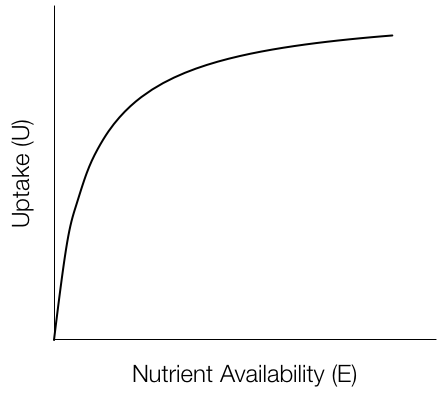
Uptake is a Michaelis-Menton function of nutrient availability limited, in part, by nutrient-specific uptake tissue surface area (roots, etc., \(SV\)):
\[U_n = \frac{S_nV_n En}{k_n + E_n}\]
with \(S_n=B_n^{2/3}\), the biomass made up of the respective nutrient.
\(V\) changes over time as the plant attempts to optimize uptake to balance the ratio in its biomass to reach an optimal value, \(Q\):
\[\frac{dV_n}{dt} = a\left[\ln(Q) - \ln\left(\frac{B_n}{B_2}\right)\right] V_n\]
Equilibrium solutions: Three Cases
Case 1: When nutrient availability is constant, the plants act as if under multiple element limitation, though responses to increased nutrients may be small due to saturation of uptake.
Case 2: When nutrients are depletable, plants act as if limited by only one nutrient (i.e., Liebig limitation), but the growth response is linear with respect to the replenishment rate \((R)\)
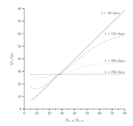
Case 3: When nutrients are a mix of constant and depletable, plants respond as in Case #2 when the depletable nutrient is limiting, but above a critical rate of replenishment, act as in Case #1, with saturating limitation of the non-depletable element.
Dynamics
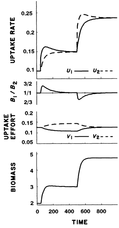
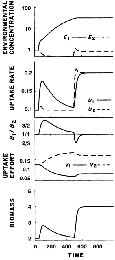
Simulations were run under this model, increasing the supply of one nutrient at \(T=50\) and a second nutrient at \(T=500\).
Case 1: With nutrients undepletable, plants increased growth in response to increases in both nutrients, in both cases falling out of the optimal balance of nutrients \((Q)\), but finding a new equilibrium at higher biomass.
Case 2: With nutrients depletable, plants experienced initial increases in growth and biomass, but returned to previous levels in order to balance nutrient levels. Only when both nutrients were added was higher biomass sustained.
Case 3: In the mixed case, plants responded as in Case #2 until \(R\) was above the critical replenishment rate, then responded as in Case #1.
Klausmeier et al. (2007)
Klausmeier et al. use a similar framework to model the dynamics of microbial growth dynamics and competition. In their model, growth under two nutrients is subject to Liebig-style limitation of nutrient concentrations \((Q)\) inside cells, while uptake into cells \((U)\) is driven by Michaelis-Menton kinetics (designated by function \(f\), which is linear with respect to \(A\), the allocation term.):
\[\frac{dQ_{n}}{dt} = f(R, A) - \mu \min \left(1 - \frac{Q_{min,n}}{Q_n}, 1-\frac{Q_{min,o}}{Q_o} \right) Q_n\]
\[\frac{dB}{dt} = \mu \min \left(1 - \frac{Q_{min,n}}{Q_n}, 1-\frac{Q_{min,o}}{Q_o} \right) B - mB\]
Optimal strategies - Static
The authors show that a species whose allocation leads to co-limitation has a continuously stable strategy (an evolutionary stable strategy that is stable on its own).
Dynamics
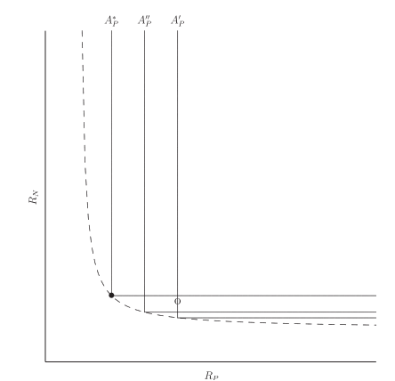
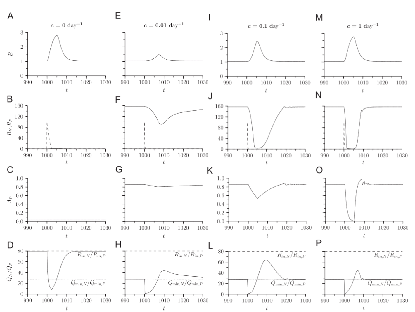
To make allocation dynamic, the authors simply change \(A\) at a constant rate so as to reach the level where both nutrients are limiting:
\[\frac{dA}{dt} = \begin{cases} c(1-A) &(P-Limited) \\ -cA &(N-limited)\\ 0 & (colimited) \end{cases} \]
The authors show two consequences of dynamic allocation. First, plankton nutrient ratios can be sensitive to time of sampling, as it can take time for biomass nutrient ratios to adjust to environmental levels. This adjustment may take longer than the change in biomass that may result from changes in nutrient levels.
Secondly, the relationship between allocation rate and growth response to nutrients is not simple. In simulations, organisms with no acclimation ability grow as quickly in response to a nutrient pulse as organisms that acclimate quickly, but slow acclimators do worse than both.
The high growth rates of slow-acclimation organisms in response to a pulse suggest that this strategy may be superior in a fluctuating environment, and in simulations, this is the case.
Rastetter (2011)
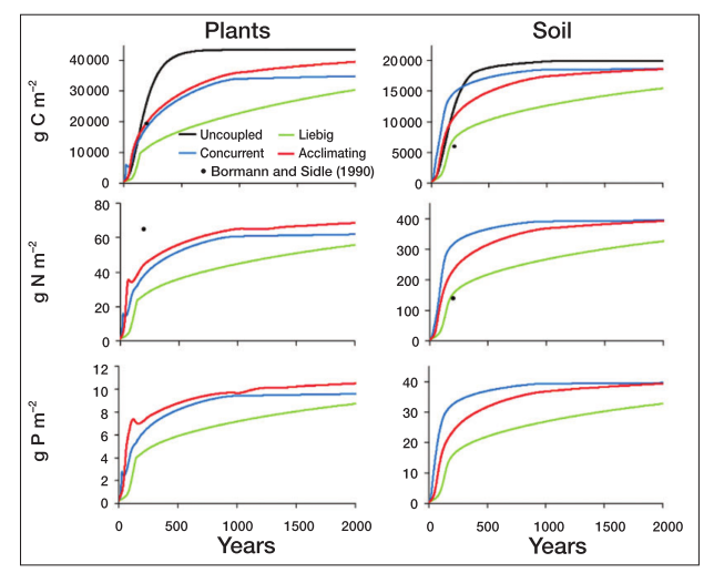
Rastetter (2011) examines the role of acclimation in ecosystem succession and in and in ecosystem response to carbon enrichment and climate change. He uses a slightly more involved ecosystem than the previous two papers (detailed in the supplmentary information), which represents plant, soil, and microbe nutrient cycling in a Douglas-fir forest. He then modifies it in four ways:
- Plants and microbe growth is driven by M-M nutrient uptake, but nutrient uptake among different nutrients are uncouples.
- Nutrient uptake is determined via Liebig’s law
- Nutrients are co-limiting, in which each nutrient’s uptake is proportional to availability of the rest, and
- Organisms adapt by allocating uptake tissue, as in Rastetter and Shaver (1992)
When simulating forest growth and succession, the uncoupled model reaches an equilibrium faster, while the Liebig model is sloweest.
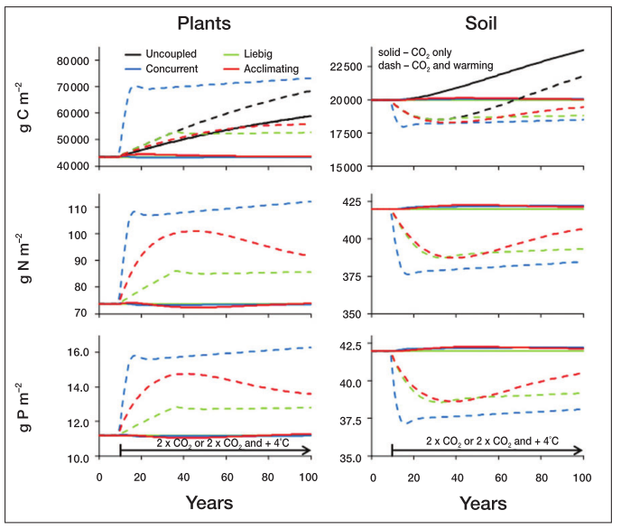
Under the climate change simulations, the concurrent limitation leads to more rapid changes following temperature and CO2 increases. The uncoupled system is the only one to change with only CO2 enrichment, though.
Some thoughts
These three papers study similar ideas, modeled at the plant organism, plankton population, and whole-forest level. Should similar mechanisms hold across these?
What limitation or adaptation mechanisms are appropriate in what models? In what cases are constant-environment v. environment-organism-feedback approaches appropriate?
References
Klausmeier, C., E. Litchman, and S. Levin. 2007. A model of flexible uptake of two essential resources.. Journal of theoretical biology 246:278–89.
Rastetter, E. B. 2011. Modeling coupled biogeochemical cycles. Frontiers in Ecology and the Environment 9:68–73.
Rastetter, E. B., and G. R. Shaver. 1992. A Model of Multiple-Element Limitation for Acclimating Vegetation. Ecology 73:1157–1174.