Last week in Davis R Users’ Group, Lauren Yamane showed us how she created and analyzed a stochastic age-structured population in R. Her examples are below. Her original scripts can be found as *.Rmd files here
A note to UC Davis students: This topic and others will be covered by Marissa Baskett and Sebastian Schreiber in their course this winter, Computational methods in population biology (ECL298)
A discrete time, age-structured model of a salmon population (semelparous) that can live to age 5, with fishing and environmental stochasticity
Parameter values
a = 60  #alpha for Beverton-Holt stock-recruitment curve
b = 0.00017  #beta for Beverton-Holt
tf = 2000  #number of time steps
N0 = c(100, 0, 0, 0, 0)  #initial population vector for 5 age classes
s = 0.28  #survival rate with fishing
e = 0.1056  #fraction of age 3 fish that spawn early (age 4 is mean spawner age)
l = 0.1056  #fraction of age 4 fish that spawn late as age 5 fish
sx = c(s, s, (s * (1 - e)), (s * (l)))  #survival vector for all ages with fishing, spawners die after spawning
t <- 1  #start off at time=1
Make a function for the age-structured matrix
# Make a function for the age-structured matrix with fishing
AgeStructMatrix_F = function(sx, a, b, tf, N0) {
    sig_r = 0.3
    ncls = length(N0)  #Number of age classes
    Nt_F = matrix(0, tf, ncls)  #Initialize output matrix with time steps as rows, age classes as columns
    Nt_F[1, ] = N0  #put initial values into first row of output matrix
    for (t in 1:(tf - 1)) {
        #for time step t in 1:1999
        Pt = (e * Nt_F[t, 3]) + ((1 - l) * Nt_F[t, 4]) + Nt_F[t, 5]  #number of spawners
        Nt_F[t + 1, 1] = ((a * Pt)/(1 + (b * Pt))) * (exp(sig_r * rnorm(1, mean = 0,
            sd = 1)))  #number of recruits with environmental stochasticity
        Nt_F[t + 1, 2:ncls] = sx * Nt_F[t, 1:(ncls - 1)]  #number of age classes 2-5
    }
    return(Nt_F)
}
Run model by calling function
Plot of time series with all 5 age classes
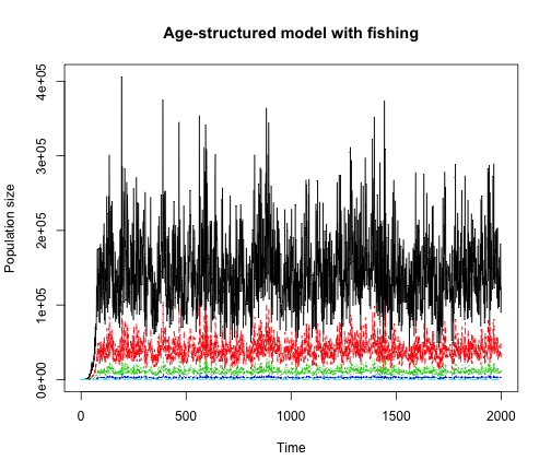
Export text file for plot with age classes
colnames(Nt_F) <- c("Recruits", "Age2", "Age3", "Age4", "Age5")  #Rename columns
write.table(Nt_F, "~/Desktop/Nt_F.txt", col.names = TRUE, row.names = FALSE,
    quote = FALSE, sep = ",")  #comma separated
Or plot of time series for total population
Nt_F_totals = rowSums(Nt_F)
plot(c(1:tf), Nt_F_totals, type = "l", xlab = "Time", ylab = "Population size",
    col = "blue")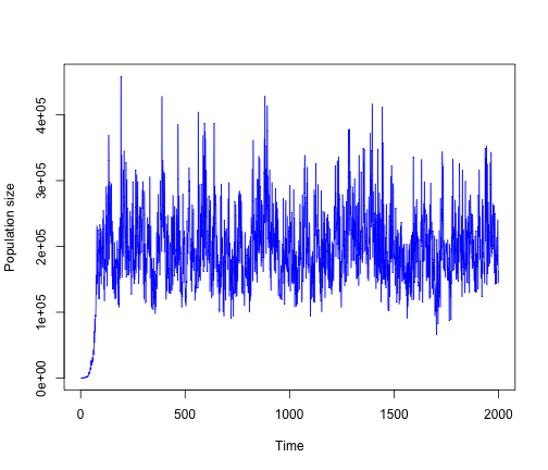
Export text file for plot with total population
write.table(Nt_F_totals, "~/Desktop/Nt_F_totals.txt", col.names = FALSE, row.names = FALSE,
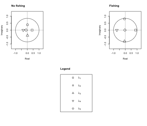
quote = FALSE, sep = ",")Stability analysis of deterministic population model
This assumes that the partial differential equations that make up the Jacobian matrix have been determined analytically. Below are the parameters that were associated with my age-structured salmon model with fishing. I can compare the stability of the population with fishing to that with no fishing
e <- 0.1056
l <- 0.1056
s <- 0.28  #survival with fishing
s_noF <- 0.85  #survival with no fishing
c <- 1/((e * (s^2) + (1 - e) * (1 - l) * (s^3) + (1 - e) * l * (s^4)))
c_noF <- 1/((e * (s_noF^2) + (1 - e) * (1 - l) * (s_noF^3) + (1 - e) * l * (s_noF^4)))
alpha <- 60
beta <- 0.00017
Fishing Jacobian
one_F <- c(0, 0, ((alpha * e)/(1 + (1/(2 * c)) * (-c + alpha + sqrt((c - alpha)^2)))^2),
    ((alpha * (1 - l))/(1 + (1/(2 * c)) * (-c + alpha + sqrt((c - alpha)^2)))^2),
    (alpha/(1 + (1/(2 * c)) * (-c + alpha + sqrt((c - alpha)^2)))^2))
two_F <- c(s, 0, 0, 0, 0)
three_F <- c(0, s, 0, 0, 0)
four_F <- c(0, 0, ((1 - e) * s), 0, 0)
five_F <- c(0, 0, 0, (l * s), 0)
jacobian_F <- rbind(one_F, two_F, three_F, four_F, five_F)
jacobian_F
# [,1] [,2] [,3] [,4] [,5]
# one_F 0.00 0.00 2.5214 21.35558 23.88
# two_F 0.28 0.00 0.0000 0.00000 0.00
# three_F 0.00 0.28 0.0000 0.00000 0.00
# four_F 0.00 0.00 0.2504 0.00000 0.00
# five_F 0.00 0.00 0.0000 0.02957 0.00Fishing Eigenvalues
ev_F <- eigen(jacobian_F)
ev1_F = c(Re(ev_F$values[1]), Im(ev_F$values[1]))
ev2_F = c(Re(ev_F$values[2]), Im(ev_F$values[2]))
ev3_F = c(Re(ev_F$values[3]), Im(ev_F$values[3]))
ev4_F = c(Re(ev_F$values[4]), Im(ev_F$values[4]))
ev5_F = c(Re(ev_F$values[5]), Im(ev_F$values[5]))
No Fishing Jacobian
one_noF <- c(0, 0, ((alpha * e)/(1 + (1/(2 * c_noF)) * (-c_noF + alpha + sqrt((c_noF -
    alpha)^2)))^2), ((alpha * (1 - l))/(1 + (1/(2 * c_noF)) * (-c_noF + alpha +
    sqrt((c_noF - alpha)^2)))^2), (alpha/(1 + (1/(2 * c_noF)) * (-c_noF + alpha +
    sqrt((c_noF - alpha)^2)))^2))
two_noF <- c(s_noF, 0, 0, 0, 0)
three_noF <- c(0, s_noF, 0, 0, 0)
four_noF <- c(0, 0, ((1 - e) * s_noF), 0, 0)
five_noF <- c(0, 0, 0, (l * s_noF), 0)
jacobian_noF <- rbind(one_noF, two_noF, three_noF, four_noF, five_noF)
jacobian_noF
# [,1] [,2] [,3] [,4] [,5]
# one_noF 0.00 0.00 0.004625 0.03917 0.0438
# two_noF 0.85 0.00 0.000000 0.00000 0.0000
# three_noF 0.00 0.85 0.000000 0.00000 0.0000
# four_noF 0.00 0.00 0.760240 0.00000 0.0000
# five_noF 0.00 0.00 0.000000 0.08976 0.0000No Fishing Eigenvalues
ev_noF <- eigen(jacobian_noF)
ev1_noF = c(Re(ev_noF$values[1]), Im(ev_noF$values[1]))
ev2_noF = c(Re(ev_noF$values[2]), Im(ev_noF$values[2]))
ev3_noF = c(Re(ev_noF$values[3]), Im(ev_noF$values[3]))
ev4_noF = c(Re(ev_noF$values[4]), Im(ev_noF$values[4]))
ev5_noF = c(Re(ev_noF$values[5]), Im(ev_noF$values[5]))

# Setup for plot, just remember to expand the plot interface first
library(plotrix)  #load plotrix
Plot the eigenvalues with legend to compare stability of both deterministic models
layout(matrix(c(1, 0, 2, 0, 3, 0), 2, 3, byrow = TRUE))  #Layout with 2 rows, 3 columns,
# the matrix tells you the number of the figure in each location. Since
# the layout is byrow, it fills the first row first and then the 2nd row
# no fishing plot
plot(ev1_noF[1], ev1_noF[2], type = "p", pch = 0, cex = 2, xlab = "Real", ylab = "Imaginary",
    xlim = c(-1.25, 1.25), ylim = c(-1.25, 1.25))
title("No fishing", adj = 0)  #plot dominant eigenvalue, with x-coordinate as real part and y-coordinate as imaginary part
draw.circle(0, 0, radius = 1, border = "black", lty = 1, lwd = 1)  #draw unit circle
points(ev2_noF[1], ev2_noF[2], pch = 1, cex = 2)  #2nd eigenvalue
points(ev3_noF[1], ev3_noF[2], pch = 2, cex = 2)  #3rd eigenvalue
points(ev4_noF[1], ev4_noF[2], pch = 6, cex = 2)  #4th eigenvalue
points(ev5_noF[1], ev5_noF[2], pch = 5, cex = 2)  #5th eigenvalue
abline(a = NULL, b = NULL, h = 0, lty = 3)
abline(a = NULL, b = NULL, v = 0, lty = 3)

# fishing plot
plot(ev1_F[1], ev1_F[2], type = "p", pch = 0, cex = 2, xlab = "Real", ylab = "Imaginary",
    xlim = c(-1.25, 1.25), ylim = c(-1.25, 1.25))
title("Fishing", adj = 0)
draw.circle(0, 0, radius = 1, border = "black", lty = 1, lwd = 1)
points(ev2_F[1], ev2_F[2], pch = 1, cex = 2)
points(ev3_F[1], ev3_F[2], pch = 2, cex = 2)
points(ev4_F[1], ev4_F[2], pch = 6, cex = 2)
points(ev5_F[1], ev5_F[2], pch = 5, cex = 2)
abline(a = NULL, b = NULL, h = 0, lty = 3)
abline(a = NULL, b = NULL, v = 0, lty = 3)

# Legend
plot(1:10, type = "n", axes = FALSE, xlab = "", ylab = "", frame.plot = TRUE)
title("Legend", adj = 0)
text(6.5, 9.5, expression(lambda[1]), cex = 1.2)
text(6.5, 7.5, expression(lambda[2]), cex = 1.2)
text(6.5, 5.5, expression(lambda[3]), cex = 1.2)
text(6.5, 3.5, expression(lambda[4]), cex = 1.2)
text(6.5, 1.5, expression(lambda[5]), cex = 1.2)
points(4.5, 9.5, pch = 0, cex = 1.3)
points(4.5, 7.5, pch = 1, cex = 1.3)
points(4.5, 5.5, pch = 2, cex = 1.3)
points(4.5, 3.5, pch = 6, cex = 1.3)
points(4.5, 1.5, pch = 5, cex = 1.3)