This is a description of the model I’ve implemented in the SODDr package, which I prepared for a presentation for the Hastings lab meeting on November 29, 2012.
Background
Sudden Oak Death (SOD) is a disease that threatens tanoak populations in California. It’s cause is an introduced pathogen, Phytophthora ramorum. Phytophthora is a water mold that spreads by wind-blown rain and fog as well as through human transport (e.g., transportation of plants). The disease has a wide host range. Mortality and transmissivity vary considerably by species.
In Northern California, SOD threatens populations of tanoak (Notholithocarpus densiflorus) and causes a long-term shift in species composition in Redwood-Bay-Tanoak forests (Metz et al. 2012). SOD causes high mortality in tanoak, with greater mortality in older, larger trees. It does not kill Bay Laurel or Redwood, but can reside in both. Bay Laurel has high transmissivity of the disease, because it broadcasts large numbers of spores from its leaves, while infected Redwoods transmit very few spores, and infected tanoaks produce a moderate amount that emerge from its bark.
Model framework
Here I describe my version of a model from Cobb et al. (2012), which simulates stand population dynamics and spread of the disease through a stand. The goal of creating and extending this model is to provide a framework to examine different treatment options to conserve tanoak, primarily by manipulating species composition and density.
The model is a discrete implementation of the continuous model described in Cobb et al. (2012). I moved to a discrete frame work in order to
- Make it easier to include stochasticity
- Fit the model to data using a hidden-Markov framework (Gimenez et al. 2012)
In addition, the model framework is designed so as to easily manipulate the species/size classes. This will allow me to simplify the structure to explore theoretical model behavior, and generate a nested set of models to fit to data.
The model has the following attributes
- Spatially explicit: Each cell on a lattice can contain trees of any species
- Multi-species: Each tree species has different parameters for growth and interaction with the disease
- Age structured: Individual trees advance through size classes which have different parameters
- SI-based: Trees may belong to a susceptible or infected class, which modifies growth and mortality parameters.
Structure
The population at time \(t\) and location \(x\) is \(\boldsymbol N_{t,x}\), which is a vector that collapses species, size , and disease categories (“classes”). Thus, for two species, each with two size categories, we have vector of eight classes at one point in space at time:
\[\boldsymbol N_{t,x} = \begin{bmatrix} a_{1,S} \\ a_{1,I} \\ a_{2,S} \\ a_{2,I} \\ b_{1,S} \\ b_{1,I} \\ b_{2,S} \\ b_{2,I} \end{bmatrix}\]
Demographic parameters vary these classes, so each demographic and epidemiological parameter is a vector. Here are the class-specific parameters:
| Parameter Vector Symbol | Description |
|---|---|
| \(\boldsymbol m\) | Probability of death per year. Varies by species, size, and disease status. |
| \(\boldsymbol b\) | Fecundity per individual per year. Varies by species and size. |
| \(\boldsymbol g\) | Probability of transition to the next size class. Varies by species and size. |
| \(\boldsymbol R'\) | Probability of recovery from disease. Varies by species. |
| \(\boldsymbol r\) | Probability of resprouting after death by disease. Varies by species. |
| \(\boldsymbol w\) | Relative space taken up by an individual tree of the class. Varies by species and size. |
Individuals do not transition between species, but they transition between size classes according to \(g\).
Individuals transition from \(S\) to \(I\) class at the rate of \(\boldsymbol \Lambda\), the class-specific force of infection. \(\Lambda\) on each class depends on both the burden of spores arriving in the cell and the class’s susceptibility to those spores. Spores arriving in the cell are calculated by summing the dispersal of spores for each infected class in the lattice, to get a vector of spore burden from each class for a location. This is multiplied by a “Who Acquires Infection From Whom” matrix (WAIFW, Anderson and May (1985)) to get \(\boldsymbol \Lambda\).
\[\boldsymbol \Lambda_{t,x} = \phi (\boldsymbol N_t, x, \boldsymbol\theta) \boldsymbol W\]
\(\phi\) is the dispersal kernel for spores from all trees to location \(x\), and \(\boldsymbol\theta\) is the vector of dispersal parameters for each class of tree. \(\boldsymbol W\) is the WAIFW matrix, which represents differing physiological susceptibility to disease as well as the vertical dispersal of spores. Vertical structure of the stand is important, as small trees being rained down upon with spores from infected tall trees are more likely to be infected than the other way around.
Trees transition from \(I\) to \(S\) by recovery at rate \(\boldsymbol R_t\). Note that \(\boldsymbol R_t\) is actually the base probability of recovery mutliplied by the probability of escaping infection until the next year:
\[R_{t} = (1-\Lambda_t) \times R'\]
Both \(S\) and \(I\) individuals are removed from the population via mortality. For some species (e.g., tanoak), this occurs at a higher rate in infected individuals
Recruitment of new individuals is density-dependent, based on shading. New recruits in the first age class sprout at a rate equal to the fecundity and population of their species in the cell, times the amount of empty space \((E_x)\) for growth:
\[E_{x,t} = 1 - \sum_i w_i N_{x,t,i}\]
In addition, a tree may resprout upon death, usually when killed by disease. This occurs with probability \(\boldsymbol r\).
With \(\Lambda, R\) and \(E\) calculated at each time step, we can create the transition matrix \(\boldsymbol L\) at time \(t\)
\[\boldsymbol L_t = \begin{bmatrix} (1-\Lambda_{1,t})(1-g_1-m_1) + b_1 E_t + r_1 m_1 & R_{2,t} (1-g_2-m_2) + b_2 E_t + r_2 m_2 & 0 & 0 & 0 & 0 & 0 & 0 \\ \Lambda_{1,t} (1-g_1-m_1) & (1-R_{2,t})(1-g_2-m_2) & 0 & 0 & 0 & 0 & 0 & 0 \\ (1-\Lambda_{1,t})g_1 & R_{2,t} g_2 & (1-\Lambda_{3,t})(1-g_3-m_3) & R_{4,t} (1-g_4-m_4) & 0 & 0 & 0 & 0 \\ \Lambda_{1,t} g_1 & (1-R_{2,t})g_2 & \Lambda_{3,t} (1-g_3-m_3) & (1-R_{4,t})(1-g_4-m_4) & 0 & 0 & 0 & 0 \\ 0 & 0 & 0 & 0 & (1-\Lambda_{5,t})(1-g_5-m_5) + b_5E + r_5m_5 & R_{6,t} (1-g_6-m_6) + b_6E_t + r_6m_6 & 0 & 0 \\ 0 & 0 & 0 & 0 & \Lambda_{5,t} (1-g_5-m_5) & (1-R_{6,t})(1-g_6-m_6) & 0 & 0 \\ 0 & 0 & 0 & 0 & (1-\Lambda_{5,t})g_5 & R_{6,t}g_6 & (1-\Lambda_{7,t})(1-g_7-m_7) & R_{8,t} (1-g_8-m_8) \\ 0 & 0 & 0 & 0 & \Lambda_{5,t} g_5 & (1-R_{6,t})g_6 & \Lambda_{7,t} (1-g_7-m_7) & (1-R_{8,t})(1-g_8-m_8) \end{bmatrix} \]
Parameterization
As implemented in Cobb et al. (2012), the model is parameterized as follows:
- 3 Species
- Tanoak - This is the species of concern. The disease causes mortality and it is only a moderate spreader. This species has 4 size classes. Mortality is lowest for middle size classes, but in infected trees an order of magnitude greater and greatest in the largest size classes. Fecundity increases with age. Resprouting 50% when killed by disease, zero otherwise.
- Bay Laurel - Litte affected by the disease, but when infected produces many spores. Only one age class.
- Redwood - Only one age class. Does not interact with the disease. Only interacts with other species via density competition.
- Dispersal to adjacent cells
- 50% of spores stay in cell of origin, 12.5% land in each of 8 adjacent cells
- Fecundities and space parameters were adjusted so as to achieve a steady state at compositions matching field measurements.
- 20 \(\times\) 20 lattice
- Disease introduced to all individuals in a center cell.
Results
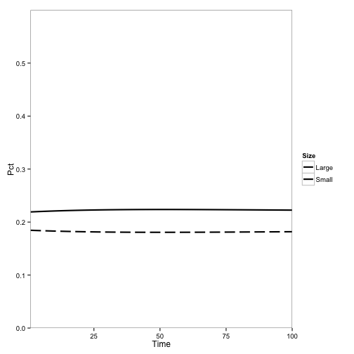
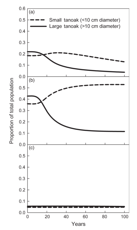
Here are the outputs of the model (as shown in my last post). They show the population of tanoak as a fraction of the total species composition, broken up into the two largest and two smallest size classes.
First, here’s the model at steady state without any disease:
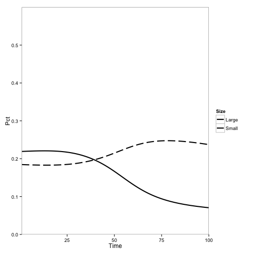
Here I introduce disease to one cell:
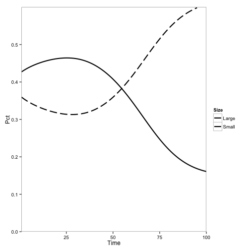
Here, the initial population is only tanoaks and redwoods, with mostly tanoaks, and disease is introduced.
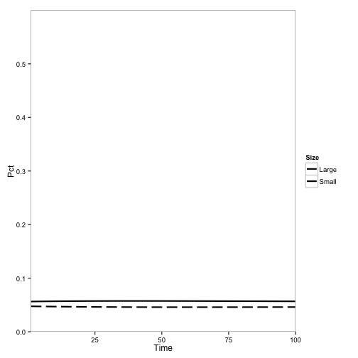
Here, the initial population is mostly redwoods, with some tanoak, and disease is introduced. No outbreak occurs:
These are pretty similar to the outputs from the Cobb et al. (2012) model. The main difference are the overall rates, which makes sense becauase I didn’t adjust the parameters for the change from continuous to discrete time:
Next steps
Now that I have the model replicated and working, I have a few tasks:
- Examine the bifurcation between stable and collapsing populations under the two-species scenario
- Do the same for three-species mixes
- Add demographic stochasticity, primarily
- Hypothesis - there’s a best density of trees for preventing collapse, that balances the risk of stochastic loss from small populations and risk of disease outbreak from big ones.
- Test robustness of results under more dispersal kernels, and heterogenous distribution of trees (clustering, etc.)
- Add an external spore source
Some areas of concern
Density Dependence: The current form of density-dependence only accounts for competition at recruitment. It’s also unstable, causing negative recruitment in some cases. Unsure how to represent this better without too much complication
- On a related note, the current “space” allocation of the trees implies that there’s greater suppression of new seedlings by the smallest and largest age classes than the middle age classes. Does this make sense?
Things to research
- Alternative distribution kernels (Chesson and Lee 2005)
- Tanoak-conifer competition literature and potential alternative models
- Tanoak recruitment distributions
Notes from Lab Meeting
Lee et al. (2001) discuss the importance of the thickness of tails Thickness of tail affects rate of spread, but for population dynamic questions often are less important. Dispersnal kernels might not matter much.
Using a simple zero/one switch for \(E\) could eliminate the artifact of negative recruitment.
Papers by Mark Lewis and Steve Pacala on spread of a population might be relevant here.
References
Anderson, R. M., and R. M. May. 1985. Age-related changes in the rate of disease transmission: implications for the design of vaccination programmes. J. Hyg. Camb.
Chesson, P., and C. T. Lee. 2005. Families of discrete kernels for modeling dispersal.. Theoretical population biology 67:241–56.
Cobb, R. C., J. A. N. Filipe, R. K. Meentemeyer, C. A. Gilligan, and D. M. Rizzo. 2012. Ecosystem transformation by emerging infectious disease: loss of large tanoak from California forests. Journal of Ecology.
Gimenez, O., J. D. Lebreton, J. M. Gaillard, R. Choquet, and R. Pradel. 2012. Estimating demographic parameters using hidden process dynamic models. Theoretical Population Biology 82:307–316.
Lee, C. T., M. F. Hoopes, J. Diehl, W. Gilliland, G. Huxel, E. V. Leaver, K. McCann, J. Umbanhowar, and A. Mogilner. 2001. Non-local concepts and models in biology.. Journal of theoretical biology 210:201–19.
Metz, M. R., K. M. Frangioso, A. C. Wickland, R. K. Meentemeyer, and D. M. Rizzo. 2012. An emergent disease causes directional changes in forest species composition in coastal California. Ecosphere 3:86.