I am working on a project with the Rizzo Lab examining the dynamics of Sudden Oak Death (SOD). I really have to write more about this, but today I’m just going to post the results of an initial exercise.
Here I attempt to replicate model results from Cobb et al. (2012). The model in that paper simulates the spread of disease and resulting tree mortality and stand dynamics in a mixed system of tanoak, bay laurel, and redwood. In this system, only tanoak and bay laurel carry the disease, and it mostly only kills tanoak, but all three species compete for space in the forest. More detail on the model found in the paper and the paper’s supplement.
I’m developing this model as an R package -"SODDr" (Sudden Oak Death Dynamics in R), to replicate this work, you can install it from github. Note that this is a very rough package and is changing.
library(devtools) # devtools enables intsallation from alternate code locations
install_github("SODDr","noamross")My model modifies the original in a few ways. First, it’s designed to be much more flexible, and make it easy to modify the number of species, size classes, and and disease parameters. Secondly, it is in a discrete- rather than continuous-time framework. This will make it easier to include stochasticity down the road, and ultimately fit it to actual data.
Setup
First, I load a CSV file of parameters
treeparms.df <- read.csv(system.file("paper_tree_parms_eq.csv", package = "SODDr"),
    stringsAsFactors = FALSE)
print(treeparms.df)
## species ageclass S.mortality I.mortality S.recruit I.recruit
## 1 1 1 0.0061 0.019 NA NA
## 2 1 2 0.0031 0.022 0.007 0.007
## 3 1 3 0.0011 0.035 0.020 0.020
## 4 1 4 0.0320 0.140 0.073 0.073
## 5 2 1 0.0200 0.020 NA NA
## 6 3 1 0.0050 0.020 NA NA
## S.transition I.transition S.resprout I.resprout recover space
## 1 0.05212 0.05212 0 0.5 0.01 NA
## 2 0.01848 0.01848 0 0.5 0.01 NA
## 3 0.01473 0.01473 0 0.5 0.01 NA
## 4 0.00000 0.00000 0 0.5 0.01 NA
## 5 0.00000 0.00000 0 0.0 0.10 1
## 6 0.00000 0.00000 0 0.0 0.10 1
## kernel.fn kernel.par1 kernel.par2 S.init I.init waifw1 waifw2
## 1 adjacent.dispersal 0.5 0.125 0.03860 0 0.33 0.33
## 2 adjacent.dispersal 0.5 0.125 0.09785 0 0.32 0.32
## 3 adjacent.dispersal 0.5 0.125 0.11379 0 0.30 0.30
## 4 adjacent.dispersal 0.5 0.125 0.04827 0 0.24 0.24
## 5 adjacent.dispersal 0.5 0.125 0.11550 0 0.30 0.30
## 6 adjacent.dispersal 0.5 0.125 0.32550 0 0.00 0.00
## waifw3 waifw4 waifw5 waifw6
## 1 0.33 0.33 1.46 0
## 2 0.32 0.32 1.46 0
## 3 0.30 0.30 1.46 0
## 4 0.24 0.24 1.46 0
## 5 0.30 0.30 1.33 0
## 6 0.00 0.00 0.00 0This data set includes all of the model parameters as defined by Cobb et al. (2012). For each species and age class, there are parameters for mortality, recruitment, transition between classes, the probability of resprouting, and recovering from disease. There are also parameters the the relative amount of space occupied by trees of each species/class.
For each species/class, the table includes a kernel function to describe dispersal of disease spores from diseased trees, and parameters for that function. The last set of columns represent the "“Who Acquires Infection From Whom” (WAIFW) matrix (Anderson and May 1985), which describes the vulnerability of each class to spores originating from others.
Note that several values, such as the space occupied by different tanoak size classes, and recruitment rates, are missing. This is because, per the original paper, I calculate these so as to parameterize the model for steady-state conditions in the absence of disease. Here I do that, using Equation 8 in the papers’ supplement:
treeparms.df <- within(treeparms.df, {
    # Calculate the relative space requirements of tanoak size classes based
    # on initial conditions
    space[1:4] <- 0.25 * (sum(S.init[1:4])/S.init[1:4])

    # Set recruitment rates to steady-state levels.  For Redwood and Bay, this
    # is simply the mortality rate divided by the density-dependence
    # coefficient at simulation start.  For tanoak, which has multiple size
    # classes, it's a but more involved

    S.recruit[5] <- S.mortality[5]/(1 - sum(S.init * space))
    I.recruit[5] <- I.mortality[5]/(1 - sum(S.init * space))
    S.recruit[6] <- S.mortality[6]/(1 - sum(S.init * space))
    I.recruit[6] <- I.mortality[6]/(1 - sum(S.init * space))

    A2 <- S.transition[1]/(S.transition[2] + S.mortality[2])
    A3 <- (S.transition[2]/(S.transition[3] + S.mortality[3])) * A2
    A4 <- (S.transition[3]/S.mortality[4]) * A3
    S.recruit[1] <- (S.transition[1] + S.mortality[1])/(1 - sum(S.init * space)) -
        (S.recruit[2] * A2 + S.recruit[3] * A3 + S.recruit[4] * A4)


    I.recruit[1] <- S.recruit[1]
    A2 <- NULL
    A3 <- NULL
    A4 <- NULL
})
The original model allows only dispersal between adjacent cells, so the parameters table calls the dispersal kernel adjacent.dispersal, and gives two parameters. This function outputs the first parameter when within the cell, the second for dispersal to adjacent cells, and zero for other cells:
## function (distance, local, adjacent)
## {
##     ifelse(distance < 0.5, local, ifelse(distance < 1.5, adjacent,
##         0))
## }
## <environment: namespace:SODDr>
Next I set up the locations in the model. These must be in the form of a matrix with the first column being site numbers, and the second being x and y coordinates. MakeLattice is a convenience function that creates a regularly spaced grid:
##      location x y
## [1,]        1 0 0
## [2,]        2 0 1
## [3,]        3 0 2
## [4,]        4 0 3
## [5,]        5 0 4
## [6,]        6 0 5
Next, I create a matrix of initial population values, which should be sized by number of locations by number of species/size classes times 2. They should be in order of the classes as they appear in the data table, but alternating \(S,I,S,I,\dots\). In this case, initial populations are uniform across the landscape and equal to the init values from the parameters table.
initial.vec = as.vector(rbind(treeparms.df$S.init, treeparms.df$I.init))
init <- matrix(data = initial.vec, nrow = nrow(locations), ncol = 2 * nrow(treeparms.df),
    byrow = TRUE)
Finally, we set the time steps for the model
Do it!
Running SODModel runs the model and generates a dataframe of population by time, species, size class, and disease status
## 'data.frame':    480000 obs. of  6 variables:
##  $ Time      : int  1 1 1 1 1 1 1 1 1 1 ...
##  $ Location  : int  1 1 1 1 1 1 1 1 1 1 ...
##  $ Species   : Factor w/ 3 levels "1","2","3": 1 1 1 1 1 1 1 1 2 2 ...
##  $ AgeClass  : Factor w/ 4 levels "1","2","3","4": 1 1 2 2 3 3 4 4 1 1 ...
##  $ Disease   : Factor w/ 2 levels "S","I": 1 2 1 2 1 2 1 2 1 2 ...
##  $ Population: num  0.0386 0 0.0978 0 0.1138 ...
Results
Here are the results, broken up by species and age class:
## Attaching package: 'plyr'

## The following object(s) are masked from 'package:twitteR':
##
## id
pop.df.totals <- ddply(pop.df, c("Time", "Disease", "Species", "AgeClass"),
summarise, TotPop = mean(Population))
dynamic.plot <- ggplot(pop.df.totals, aes(x = Time, y = TotPop, fill = Disease,
color = AgeClass)) + geom_area(position = "stack", alpha = 0.6) + facet_grid(~Species)
dynamic.plot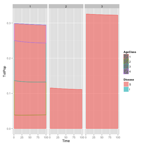
The plot shows that this isn’t quite steady-state, I suspect because of some rounding errors in copying parameters from the paper.
We can make a plot in the style of Cobb et al. (2012), showing only the populations of small and large tanoaks as a proportion of the total population:
paper.df <- ddply(transform(pop.df.totals, Size = ifelse(AgeClass == "1" | AgeClass ==
    "2", "Small", "Large")), c("Time", "Species", "Size"), summarise, SizePop = sum(TotPop))
paper.df <- ddply(paper.df, "Time", transform, Pct = SizePop/sum(SizePop))
paper.plot <- ggplot(subset(paper.df, Species == 1), aes(x = Time, y = Pct,
    lty = Size)) + geom_line(lwd = 1) + scale_y_continuous(limits = c(0, 0.6),
    expand = c(0, 0)) + scale_x_continuous(expand = c(0, 0)) + scale_linetype_manual(values = c(1,
    5)) + theme_bw() + theme(panel.grid.major = element_blank(), panel.grid.minor = element_blank())
paper.plot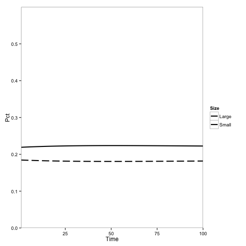
Now, let’s change the initial conditions to include disease and see what happens. I change the populations of tanoak and bay in one pixel to infectious instead of susceptible and run the model:
init[190, 2] <- init[190, 1]
init[190, 1] <- 0
init[190, 10] <- init[190, 9]
init[190, 9] <- 0
pop2.df <- SODModel(treeparms.df, locations, time.steps, init)
pop2.df.totals <- ddply(pop2.df, c("Time", "Disease", "Species", "AgeClass"),
    summarise, TotPop = mean(Population))
paper2.df <- ddply(transform(pop2.df.totals, Size = ifelse(AgeClass == "1" |
    AgeClass == "2", "Small", "Large")), c("Time", "Species", "Size"), summarise,
    SizePop = sum(TotPop))
paper2.df <- ddply(paper2.df, "Time", transform, Pct = SizePop/sum(SizePop))
paper2.plot <- ggplot(subset(paper2.df, Species == 1), aes(x = Time, y = Pct,
    lty = Size)) + geom_line(lwd = 1) + scale_y_continuous(limits = c(0, 0.6),
    expand = c(0, 0)) + scale_x_continuous(expand = c(0, 0)) + scale_linetype_manual(values = c(1,
    5)) + theme_bw() + theme(panel.grid.major = element_blank(), panel.grid.minor = element_blank())
paper2.plot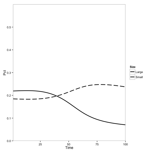
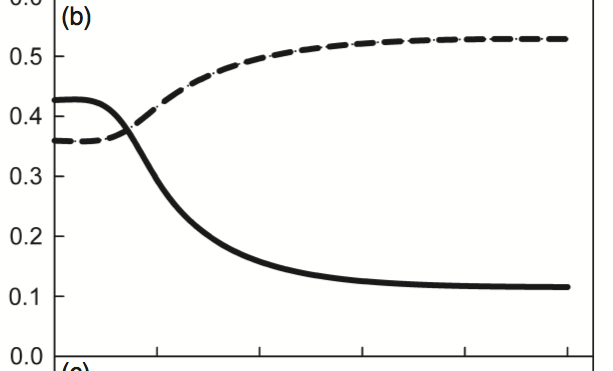
Qualitatively, this looks a lot like the original result:
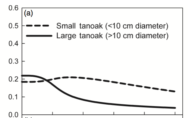
The main difference is the overall rate of change, which is expected because I haven’t corrected any parameters for the change from continuous to discrete time.
Now I simulate a scenario with mostly tanoak, some redwood, and no bay laurel, with disease, using the parameters previously calulated for the steady state without disease:
treeparms.df$S.init <- c(0.7 * treeparms.df$S.init[1:4]/sum(treeparms.df$S.init[1:4]),
    0, 0.19)

initial.vec = as.vector(rbind(treeparms.df$S.init, treeparms.df$I.init))
init <- matrix(data = initial.vec, nrow = nrow(locations), ncol = 2 * nrow(treeparms.df),
    byrow = TRUE)

init[190, 2] <- init[190, 1]
init[190, 1] <- 0
init[190, 10] <- init[190, 9]
init[190, 9] <- 0

treeparms.df <- within(treeparms.df, {
    # Calculate the relative space requirements of tanoak size classes based
    # on initial conditions
    space[1:4] <- 0.25 * (sum(S.init[1:4])/S.init[1:4])

    # Set recruitment rates to steady-state levels.  For Redwood and Bay, this
    # is simply the mortality rate divided by the density-dependence
    # coefficient at simulation start.  For tanoak, which has multiple size
    # classes, it's a but more involved

    S.recruit[5] <- S.mortality[5]/(1 - sum(S.init * space))
    I.recruit[5] <- I.mortality[5]/(1 - sum(S.init * space))
    S.recruit[6] <- S.mortality[6]/(1 - sum(S.init * space))
    I.recruit[6] <- I.mortality[6]/(1 - sum(S.init * space))

    A2 <- S.transition[1]/(S.transition[2] + S.mortality[2])
    A3 <- (S.transition[2]/(S.transition[3] + S.mortality[3])) * A2
    A4 <- (S.transition[3]/S.mortality[4]) * A3
    S.recruit[1] <- (S.transition[1] + S.mortality[1])/(1 - sum(S.init * space)) -
        (S.recruit[2] * A2 + S.recruit[3] * A3 + S.recruit[4] * A4)


    I.recruit[1] <- S.recruit[1]
    A2 <- NULL
    A3 <- NULL
    A4 <- NULL
})

pop3.df <- SODModel(treeparms.df, locations, time.steps, init)
pop3.df.totals <- ddply(pop3.df, c("Time", "Disease", "Species", "AgeClass"),
    summarise, TotPop = mean(Population))
paper3.df <- ddply(transform(pop3.df.totals, Size = ifelse(AgeClass == "1" |
    AgeClass == "2", "Small", "Large")), c("Time", "Species", "Size"), summarise,
    SizePop = sum(TotPop))
paper3.df <- ddply(paper3.df, "Time", transform, Pct = SizePop/sum(SizePop))
paper3.plot <- ggplot(subset(paper3.df, Species == 1), aes(x = Time, y = Pct,
    lty = Size)) + geom_line(lwd = 1) + scale_y_continuous(limits = c(0, 0.6),
    expand = c(0, 0)) + scale_x_continuous(expand = c(0, 0)) + scale_linetype_manual(values = c(1,
    5)) + theme_bw() + theme(panel.grid.major = element_blank(), panel.grid.minor = element_blank())
paper3.plot
## Warning: Removed 5 rows containing missing values (geom_path).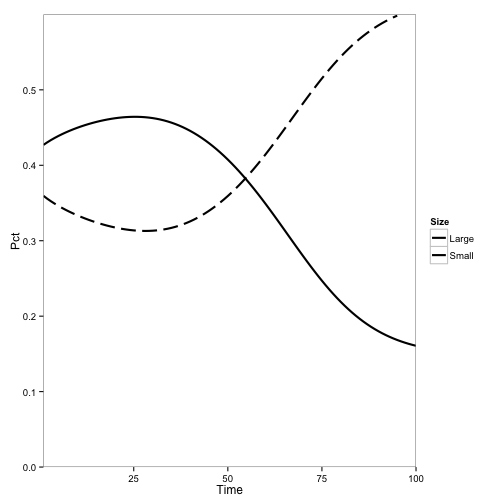
Again, qualitatively similar to the original results:
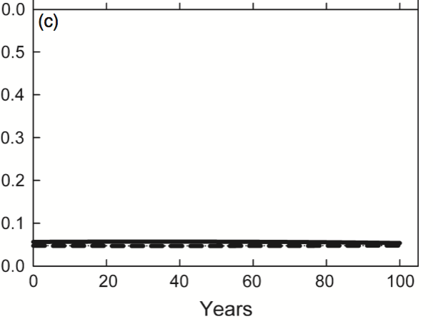
Finally, I simulate the “Mostly Redwood” scenario:
treeparms.df$S.init <- c(0.08 * treeparms.df$S.init[1:4]/sum(treeparms.df$S.init[1:4]),
    0, 0.69)

initial.vec = as.vector(rbind(treeparms.df$S.init, treeparms.df$I.init))
init <- matrix(data = initial.vec, nrow = nrow(locations), ncol = 2 * nrow(treeparms.df),
    byrow = TRUE)

init[190, 2] <- init[190, 1]
init[190, 1] <- 0
init[190, 10] <- init[190, 9]
init[190, 9] <- 0

treeparms.df <- within(treeparms.df, {
    # Calculate the relative space requirements of tanoak size classes based
    # on initial conditions
    space[1:4] <- 0.25 * (sum(S.init[1:4])/S.init[1:4])

    # Set recruitment rates to steady-state levels.  For Redwood and Bay, this
    # is simply the mortality rate divided by the density-dependence
    # coefficient at simulation start.  For tanoak, which has multiple size
    # classes, it's a but more involved

    S.recruit[5] <- S.mortality[5]/(1 - sum(S.init * space))
    I.recruit[5] <- I.mortality[5]/(1 - sum(S.init * space))
    S.recruit[6] <- S.mortality[6]/(1 - sum(S.init * space))
    I.recruit[6] <- I.mortality[6]/(1 - sum(S.init * space))

    A2 <- S.transition[1]/(S.transition[2] + S.mortality[2])
    A3 <- (S.transition[2]/(S.transition[3] + S.mortality[3])) * A2
    A4 <- (S.transition[3]/S.mortality[4]) * A3
    S.recruit[1] <- (S.transition[1] + S.mortality[1])/(1 - sum(S.init * space)) -
        (S.recruit[2] * A2 + S.recruit[3] * A3 + S.recruit[4] * A4)


    I.recruit[1] <- S.recruit[1]
    A2 <- NULL
    A3 <- NULL
    A4 <- NULL
})

pop4.df <- SODModel(treeparms.df, locations, time.steps, init)
pop4.df.totals <- ddply(pop4.df, c("Time", "Disease", "Species", "AgeClass"),
    summarise, TotPop = mean(Population))
paper4.df <- ddply(transform(pop4.df.totals, Size = ifelse(AgeClass == "1" |
    AgeClass == "2", "Small", "Large")), c("Time", "Species", "Size"), summarise,
    SizePop = sum(TotPop))
paper4.df <- ddply(paper4.df, "Time", transform, Pct = SizePop/sum(SizePop))
paper4.plot <- ggplot(subset(paper4.df, Species == 1), aes(x = Time, y = Pct,
    lty = Size)) + geom_line(lwd = 1) + scale_y_continuous(limits = c(0, 0.6),
    expand = c(0, 0)) + scale_x_continuous(expand = c(0, 0)) + scale_linetype_manual(values = c(1,
    5)) + theme_bw() + theme(panel.grid.major = element_blank(), panel.grid.minor = element_blank())
paper4.plot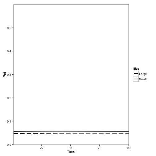
Success! Same results as the original:
Now, for fun, let’s make an animation of how the disease progresses through the stand. I will use the “Mostly Tanoak” scenario", and plot the adult population as intensity, and the fraction of trees diseased as hue.
tanspc <- subset(pop3.df, Species == 1)
tanspc$Species <- NULL
tanspc <- ddply(tanspc, c("Time", "Location"), function(x) {
    data.frame(TotTan = sum(x$Population[which(x$AgeClass == "3" | x$AgeClass ==
        "4")]), FracDisease = sum(x$Population[which(x$Disease == "I" & (x$AgeClass ==
        "3" | x$AgeClass == "4"))])/sum(x$Population[which(x$AgeClass == "3" |
        x$AgeClass == "4")]))
})
tanspc <- merge(tanspc, as.data.frame(locations), by.x = "Location", by.y = "location")
dis.limits <- c(min(tanspc$FracDisease), max(tanspc$FracDisease))
pop.limits <- c(min(tanspc$TotTan), max(tanspc$TotTan))
require(animation)
## Loading required package: animationani.options(nmax = 50, loop = TRUE, interval = 0.2)
for (time in time.steps) {
print(ggplot(data = subset(tanspc, Time == time), aes(x = x, y = y, fill = FracDisease,
alpha = TotTan)) + geom_tile() + scale_alpha(name = "TanoakPopulation",
limits = c(0, 0.4), breaks = seq(0, 0.4, 0.1)) + scale_fill_continuous(name = "Fraction Diseased",
limits = c(0, 1), breaks = seq(0, 1, 0.25), low = "#408000", high = "#FF8000") +
theme(rect = element_blank(), line = element_blank()))
}References
Anderson, R. M., and R. M. May. 1985. Age-related changes in the rate of disease transmission: implications for the design of vaccination programmes. J. Hyg. Camb.
Cobb, R. C., J. a. N. Filipe, R. K. Meentemeyer, C. a Gilligan, and D. M. Rizzo. 2012. Ecosystem transformation by emerging infectious disease: loss of large tanoak from California forests. Journal of Ecology.