Dave Harris on Maximum Likelihood Estimation

At our last Davis R Users’ Group meeting of the quarter, Dave Harris gave a talk on how to use the bbmle package to fit mechanistic models to ecological data. Here’s his script, which I ran throgh the spin function in knitr:

# Load data
library(emdbook)

## Loading required package: MASS Loading required package: lattice

library(bbmle)

## Loading required package: stats4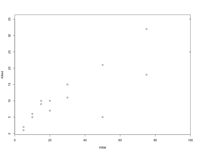

data(ReedfrogFuncresp)
plot(ReedfrogFuncresp, xlim = c(0, 100), xaxs = "i")

Statistical models are stories about how the data came to be. The deterministic part of the story is a (slightly mangled) version of what you’d expect if the predators followed a Type II functional response:

Holling’s Disk equation for Type II Functional Response

a is attack rate
h is handling time

disk = function(N, a, h) {
    N * a/(1 + N * a * h)
}

We can plot different values of a and h to see what kinds of data this model would generate on average:

plot(ReedfrogFuncresp, xlim = c(0, 100), xaxs = "i")
# a = 3, h = 0.05 (black) rises too quickly, saturates too quickly
curve(disk(x, a = 3, h = 0.05), add = TRUE, from = 0, to = 100)
# a = 2, h = 0.02 (red) still rises too quickly
curve(disk(x, 2, 0.02), add = TRUE, from = 0, to = 100, col = 2)
# a = 0.5, h = 0.02 (blue) looks like a plausible data-generating process
curve(disk(x, 0.5, 0.02), add = TRUE, from = 0, to = 100, col = 4)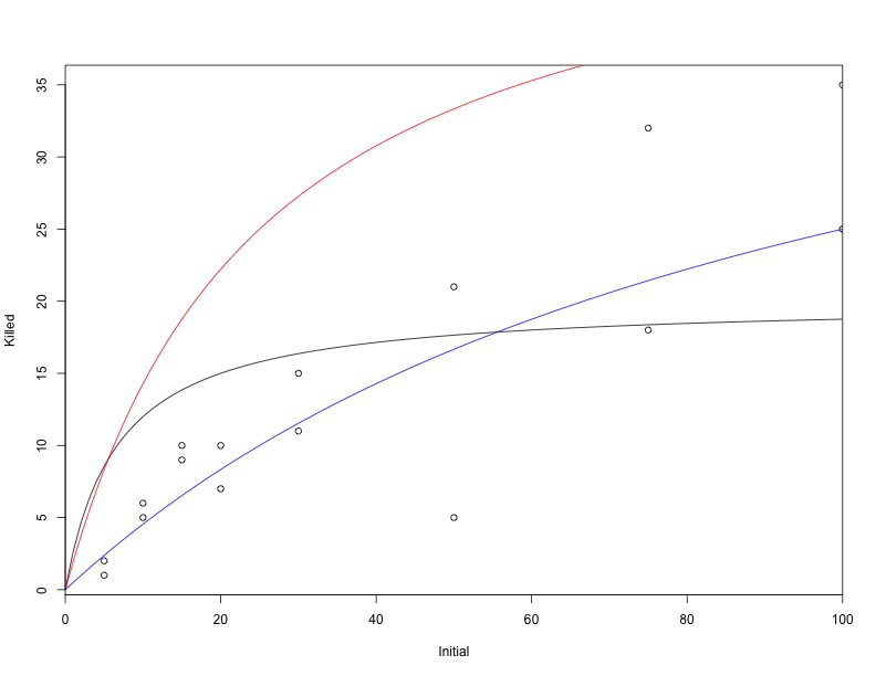

The blue curve looks plausible, but is it optimal? Does it tell the best possible story about how the data could have been generated?

In order to tell if it’s optimal, we need to pick something to optimize. Usually, that will be the log-likelihood–i.e. the log-probability that the data would have come out this way if the model were true. Models with higher probabilities of generating the data we observed therefore have higher likelihoods. For various arbitrary reasons, it’s common to minimize the negative log-likelihood rather than maximizing the positive log-likelihood. So let’s write a function that says what the log-likelihood is for a given pair of a and h.

The log-likelihood is the sum of log-probabilities from each data point. The log-probability for a data point is (in this contrived example) drawn from a binomial (“coin flip”) distribution, whose mean is determined by the disk equation.

NLL = function(a, h) {
    -sum(dbinom(ReedfrogFuncresp$Killed, size = ReedfrogFuncresp$Initial, prob = disk(ReedfrogFuncresp$Initial,
        a, h)/ReedfrogFuncresp$Initial, log = TRUE))
}

We can optimize the model with the mle2 function. It finds the lowest value for the negative log-likelihood (i.e. the combination of parameters with the highest positive likelihood, or the maximum likelihood estimate).

The NLL function we defined above requires starting values for a and h. Let’s naively start them at 1, 1

fit = mle2(NLL, start = list(a = 1, h = 1))

## Warning: NaNs produced Warning: NaNs produced Warning: NaNs produced
## Warning: NaNs produced Warning: NaNs produced Warning: NaNs produced
## Warning: NaNs produced Warning: NaNs produced Warning: NaNs produced
## Warning: NaNs produced Warning: NaNs produced Warning: NaNs produced
## Warning: NaNs produced Warning: NaNs produced Warning: NaNs produced
## Warning: NaNs produced Warning: NaNs produced Warning: NaNs produced

You’ll probably get lots of warnings about NaNs. That’s just the optimization procedure complaining because it occasionally tries something impossible (such as a set of parameters that would generate a negative probability of being eaten). In general, these warnings are nothing to worry about, since the optimization procedure will just try better values. But it’s worth checking to make sure that there are no other warnings or problems by calling warnings() after you fit the model.

# print out the results
fit

##
## Call:
## mle2(minuslogl = NLL, start = list(a = 1, h = 1))
##
## Coefficients:
##       a       h
## 0.52652 0.01666
##
## Log-likelihood: -46.72


# a bit more information:
summary(fit)

## Maximum likelihood estimation
##
## Call:
## mle2(minuslogl = NLL, start = list(a = 1, h = 1))
##
## Coefficients:
##   Estimate Std. Error z value   Pr(z)    
## a  0.52652    0.07112    7.40 1.3e-13 ***
## h  0.01666    0.00488    3.41 0.00065 ***
## ---
## Signif. codes:  0 '***' 0.001 '**' 0.01 '*' 0.05 '.' 0.1 ' ' 1
##
## -2 log L: 93.44

coef(fit)

##       a       h
## 0.52652 0.01666

Here’s the curve associated with the most likely combination of a and h (thick black line).

plot(ReedfrogFuncresp, xlim = c(0, 100), xaxs = "i")
curve(disk(x, a = coef(fit)["a"], h = coef(fit)["h"]), add = TRUE, lwd = 4,
    from = 0, to = 100)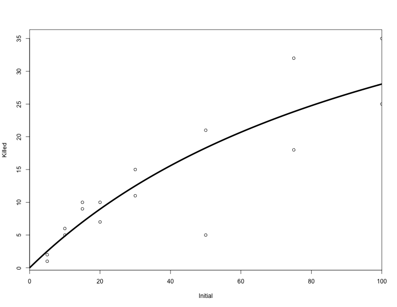

The rethinking package has a few convenient functions for summarizing and visualizing the output of an mle2 object. It’s not on CRAN, but you can get it from the author’s website or from github.

library(rethinking)

## Attaching package: 'rethinking'
##
## The following object is masked _by_ '.GlobalEnv':
##
## x

precis(fit)

##   Estimate S.E. 2.5% 97.5%
## a     0.53 0.07 0.39  0.67
## h     0.02 0.00 0.01  0.03

We can also visualize a distribution of estimates that are reasonably consistent with the observed data using the sample.naive.posterior function:

plot(sample.naive.posterior(fit), pch = ".")

# Add a red dot for the maximum likelihood estimate:
points(as.data.frame(as.list(coef(fit))), col = 2, pch = 20)

# Add a blue dot for our earlier guess:
points(0.5, 0.02, col = 4, pch = 20)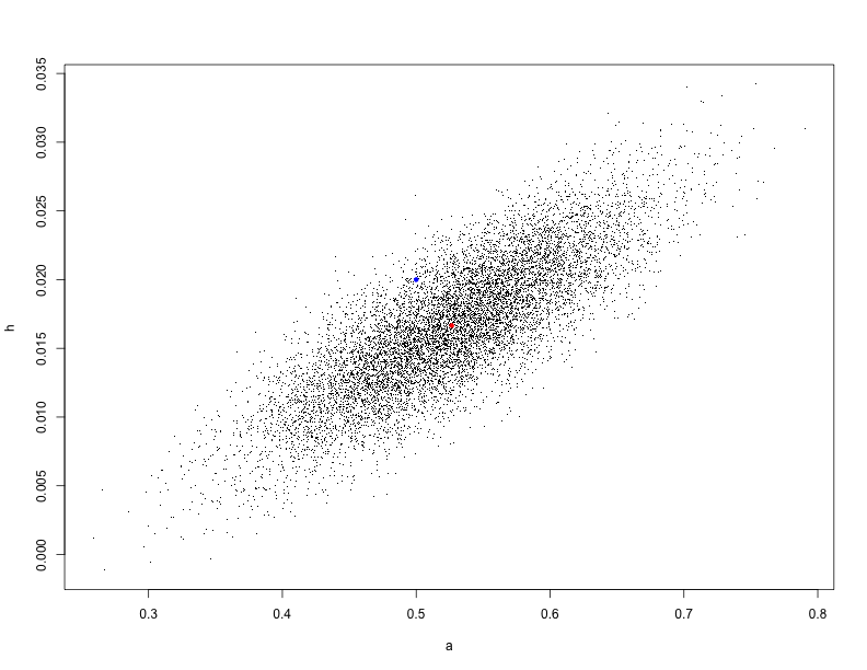

A Big digression about confidence intervals

Our earlier guess falls inside the cloud of points, so even though it’s not as good as the red point, it’s still plausibly consistent with the data.

Note that the ranges of plausible estimates for the two coefficients are correlated: This makes sense if you think about it: if the attack rate is high, then there needs to be a large handling time between attacks or else too many frogs would get eaten.

Where did this distribution of points come from? mle2 objects, like many models in R, have a variance/covariance matrix that can be extracted with the vcov() function.

vcov(fit)

##           a         h
## a 0.0050584 2.859e-04
## h 0.0002859 2.384e-05

The variance terms (along the diagonal) describe mle2’s uncertainty about the values. The covariance terms (other entries in the matrix) describe how uncertainty in one coefficient relates to uncertainty in the other coefficient.

This graph gives an example:

curve(dnorm(x, sd = 1/2), from = -5, to = 5, ylab = "likelihood", xlab = "estimate")
curve(dnorm(x, sd = 3), add = TRUE, col = 2)

The black curve shows a model with low variance for its estimate. This means that the likelihood would fall off quickly if we tried a bad estimate, and we can be reasonably sure that the data was generated by a value in a fairly narrow range. The model associated with the red curve is much less certain: the parameter could be very different from the optimal value and the likelihood wouldn’t drop much.

Here’s another way to visualize the decline in likelihood as you move away from the best estimate:

plot(profile(fit))

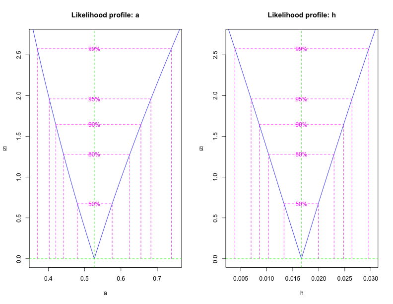
Keep in mind that all of this is based on a Gaussian approximation. It works well when you have lots of data and you aren’t estimating something near a boundary. Since h is near its minimum value (at zero), there’s some risk that the confidence intervals are inaccurate. Markov chain Monte Carlo can provide more accurate estimates, but it’s also slower to run.

Where does the vcov matrix come from? From a matrix called the Hessian. It describes the curvature of the likelihood surface, i.e. how quickly the log-likelihood falls off as you move away from the optimum.

Sometimes the Hessian is hard to estimate and causes problems, so we can run the model without it:

fit.without.hessian = mle2(NLL, start = list(a = 1, h = 1), skip.hessian = TRUE)

## Warning: NaNs produced Warning: NaNs produced Warning: NaNs produced
## Warning: NaNs produced Warning: NaNs produced Warning: NaNs produced
## Warning: NaNs produced Warning: NaNs produced Warning: NaNs produced
## Warning: NaNs produced Warning: NaNs produced Warning: NaNs produced
## Warning: NaNs produced Warning: NaNs produced Warning: NaNs produced
## Warning: NaNs produced Warning: NaNs produced Warning: NaNs produced

When there’s no Hessian, there aren’t any confidence intervals, though.

precis(fit.without.hessian)

##   Estimate S.E. 2.5% 97.5%
## a     0.53   NA   NA    NA
## h     0.02   NA   NA    NA

(End digression)

More about `mle2`

Under the hood, mle2 uses a function called optim:

`?`(optim)

It’s worth noting that most of the optimization methods used in optim (and therefore in mle2) only do a local optimization. So if your likelihood surface has multiple peaks, you may not find the right one.

mle2 also has a convenient formula inferface that can eliminate the need to write a whole likelihood function from scratch. Let’s take a look with some data found in ?mle2

x = 0:10
y = c(26, 17, 13, 12, 20, 5, 9, 8, 5, 4, 8)
d = data.frame(x, y)

Here, we’re fitting a Poisson model that depends on an intercept term plus a linear term. The exp() is mainly there to make sure that the value of lambda doesn’t go negative, which isn’t allowed (it would imply a negative number of occurrences for our outcome of interest).

fit0 = mle2(y ~ dpois(lambda = exp(intercept + slope * x)), start = list(intercept = mean(y),
    slope = 0), data = d)

Note that mle2 finds its values for x and y from the data term and that we’re giving it starting values for the slope and intercept. In general, it’s useful to start the intercept at the mean value of y and the slope terms at 0, but it often won’t matter much.

Prior information

Recall that our estimates of a and h are positively correlated: the data could be consistent with either a high attack rate and a high handling time OR with a low attack rate and a low handling time.

Suppose we have prior information about tadpole/dragonfly biology that suggests that these parameters should be on the low end. We can encode this prior information as a prior distribution on the parameters. Then mle2 won’t climb the likelihood surface. It will climb the surface of the Bayesian posterior (or if you’re frequentist, it will do a penalized or constrained optimization of the likelihood).

Here’s a negative log posterior that tries to keep the values of a and h small while still being consistent with the data:

negative.log.posterior = function(a, h) {
    NLL(a, h) - dexp(a, rate = 10, log = TRUE) - dexp(h, rate = 10, log = TRUE)
}

We optimize it exactly as before

fit2 = mle2(negative.log.posterior, start = list(a = 1, h = 1))

## Warning: NaNs produced Warning: NaNs produced Warning: NaNs produced
## Warning: NaNs produced Warning: NaNs produced Warning: NaNs produced
## Warning: NaNs produced Warning: NaNs produced Warning: NaNs produced
## Warning: NaNs produced Warning: NaNs produced Warning: NaNs produced
## Warning: NaNs produced Warning: NaNs produced Warning: NaNs produced
## Warning: NaNs produced Warning: NaNs produced Warning: NaNs produced
## Warning: NaNs produced Warning: NaNs produced Warning: NaNs produced
## Warning: NaNs produced Warning: NaNs produced Warning: NaNs produced
## Warning: NaNs produced Warning: NaNs produced Warning: NaNs produced
## Warning: NaNs produced Warning: NaNs produced Warning: NaNs produced
## Warning: NaNs produced

Sure enough, the coefficients are a bit smaller

coef(fit)  # MLE

##       a       h
## 0.52652 0.01666

coef(fit2)  # MAP estimate

##       a       h
## 0.47931 0.01375

← The null model for age effects with overdispersed infection | All posts | Printing R help files in the console or in knitr documents →

Dave Harris on Maximum Likelihood Estimation

June 17, 2013

A Big digression about confidence intervals

A somewhat-related digression:

More about mle2

Prior information

More about `mle2`