Here’s a little thought exercise I did that has caused me to go back and restart my Sudden Oak Death modeling in a new framework. Feedback welcome. I’m especially interested in relevant literature – I haven’t found many good examples of macroparasite/multiple infection models with age structure.
Introduction
Cobb et al. (2012) develop two models of forest stand demography in the face of Sudden Oak Death. The first, a statistical survival model, estimated the rates of infection and time-to-mortality as functions of density of infected trees and tree size. The second, an \(SI\) model, projected stand composition over time using parameters from the first.
I’ve been realizing is that the observed data and the first model may not square with the second model. In an \(SI\) model, all infected hosts are the same and, at least as implemented in this paper, infected trees have a constant rate of mortality. But if you look at the bottom-right portion of the figure below, you’ll see that the rate of mortality is strongly influenced by the number of infected hosts.

Richard and I discussed what might be driving this pattern, and think it might be due to the fact that trees can be infected mutiple times. Phytophthora ramorum doesn’t travel throughout a tree once infecting, but instead causes local lesions on leaves and local cankers on stems. A tree can accumulate more of these as more spores land on it. Thus, it may not be appropriate to represent infection as a binary state.
It’s also possible that multiple infection is driving another pattern. The upper-right panel above shows that there are strong size effects on mortality. It’s certainly possible that larger (or older) trees are more physiologically vulnerable to the disease. However, I think part of this may be due to the fact that larger trees have been around longer, and thus have had more time to acquire infections.
I’m exploring these hypotheses using a model adapted from Anderson and May (1978). This is a macroparasite model that explicitly considers the number of parasites in each host. My model takes its basic structure and applies it to two explicit size classes of organisms, in this case applied to trees:
\[\begin{aligned} \frac{dJ}{dt} &= A f_A \left(1 - \frac{J+A}{K} \right) + J \left(f_J \left(1 - \frac{J+A}{K} \right) - d_J - g\right) - \alpha P_J \\ \frac{dA}{dt} &= J g - A d_A - \alpha P_A \\ \frac{dP_J}{dt} &= \lambda \frac{J}{K} (P_J + P_A) - P_J \left(d_J + \mu + g + \alpha \left(1 + \frac{P_J}{J} \right) \right) \\ \frac{dP_A}{dt} &= \lambda \frac{A}{K} (P_J + P_A) + P_J g - P_A \left(d_A + \mu + \alpha \left(1 + \frac{P_A}{A} \right) \right) \end{aligned}\]
Here \(J\) and \(A\) are the population of juvenile and adult trees. There’s only two size classes for simplicity, though there’s no reason this can’t be extended to more. \(P_J\) and \(P_A\) are the total numbers of infections amongst those trees. Here’s a table of the parameters:
| Parameter | Description |
|---|---|
| \(f_J, f_J\) | Fecundity of the size class |
| \(d_J, d_A\) | Mortality rate of the size class |
| \(g\) | Rate at which juveniles become adults |
| \(\alpha\) | Amount by which a single infection increases the mortality rate |
| \(\mu\) | Rate at which trees recover from infections (ignored here) |
| \(K\) | Carrying capacity |
| \(\lambda\) | Rate at which new infections are created by a single infection. |
Some notes on the model: These equations assume that infections are completely randomly (Poisson) distributed amongst the hosts. This is unrealistic; due to spatial structure and other processes, the distribution is probably overdispersed. Secondly, unlike the Anderson and May (1978) model, there’s density dependence in recruitment of new juveniles – shading out of new recruits. Finally, transmission is density-dependent. I assume a spore’s chance of hitting a tree is proportional to the amount of space (carrying capacity) that the tree takes up.
Parameterizing and Running the Model
I define the equations and parameters in R:
model <- function(t, y, parms) {
  list2env(as.list(y), environment())
  list2env(as.list(parms), environment())
  dJ <- A*f_a*(1 - (J+A)/K) + J * (f_j*(1 - (J+A)/K) - d_j - g) - alpha * PJ
  dA <- J*g - (A * d_a) - alpha * PA
  dPJ <- lambda * (PJ + PA) * J/K - PJ*(d_j + mu + g + alpha*(1 + PJ/J))
  dPA <- lambda * (PJ + PA) * A/K + PJ * g - PA*(d_a + mu + alpha*(1 + PA/A))
  return(list(c(dJ=dJ, dA=dA, dPJ=dPJ, dPA=dPA),
              c(dJ=dJ, dA=dA, dPJ=dPJ, dPA=dPA)))
}

parms <- c(
  f_j=0.01,
  f_a=0.01,
  g=0.1,
  d_j=0.005,
  d_a=0.005,
  alpha=0.05,
  lambda=0.3,
  K=50,
  mu=0.00
  )
Note from the parameters that here the juvenile and adult trees are exactly the same in their demographic variables, their contribution to density dependence and their response to disease. That is why I call this a “null model for age effects”; any differences between the behavior of the size classes will be due to structural effects of the model. Namely, that some trees carry disease as they move from juvenile to adult size class.
The parameters are selected to be somewhat realistic for tanoak and based on Cobb et al. (2012). Effectively, the juvenile class contains trees with <1 cm diameter and adults are anything larger. The carrying capacity (\(K=50\)) is about equal to the stand density of many in the plots the Cobb et al. (2012) data set.
I initiate the model with tree populations at their disease-free steady state, and with an average of 0.1 infection per tree. Note that the steady state has a high proportion of adults due to the parameterization. Since density dependence in the model only affects recruitment of new juveniles, their population is limited by the natural death rate of adults.
A_ss = with(as.list(parms), K/(d_a/g + 1))
J_ss = with(as.list(parms), K - A_ss)
init <- c(J=J_ss, A=A_ss, PJ=0.1*J_ss, PA=0.1*A_ss)
Now I run the model and calculate some relevant values that I’ll explain when I plot them:
require(deSolve)
require(reshape2)
out <- as.data.frame(lsoda(y=init, times=1:100, func=model, parms=parms))
df <- as.data.frame(out)
names(df)[1] <- "Time"

df <- within(df, {
  list2env(as.list(parms), environment())
  pctJ <- J/(J + A)
  pctA <- A/(J + A)
  nJ <- PJ / J
  nA <- PA / A
  J.inf <- 1 - exp(-nJ)
  A.inf <- 1 - exp(-nA)
  Inf.dens <- (J*J.inf + A*A.inf)
  J.mort <- d_j + alpha * PJ /(J * J.inf)
  A.mort <- d_a + alpha * PA / (A * A.inf)
  J.yrs <- 1/J.mort
  A.yrs <- 1/A.mort
  J.infrate <- 1 - exp(-lambda * (PJ + PA) * J * exp(-PJ/J) / K)
  A.infrate <- 1 - exp(-lambda * (PJ + PA) * A * exp(-PA/A) / K)
  J.infyrs <- 1/J.infrate
  A.infyrs <- 1/A.infrate
  rm(list=names(parms))
})

df <- df[,sort(names(df), decreasing=TRUE)]

mdf <- melt(df, id.vars=c("Time", "Inf.dens"), variable.name="Class",
            value.name="Population")
Results and Discussion
OK, so what does this look like? First, I plot the absolute and relative population sizes over time:
require(ggplot2)
require(gridExtra)
JAlab <- scale_color_discrete(labels=c("Small Trees","Big Trees"))
p1 <- ggplot(subset(mdf, Class %in% c("J", "A")),
             aes(x=Time, y=Population, col=Class)) +
      geom_line(lwd=1) + theme_nr + ylab("Population") + JAlab
p2 <- ggplot(subset(mdf, Class %in% c("pctJ", "pctA")),
             aes(x=Time, y=Population, col=Class)) +
      geom_line(lwd=1) + theme_nr + ylab("Fraction of Population") + JAlab
grid.arrange(p1, p2, nrow=2)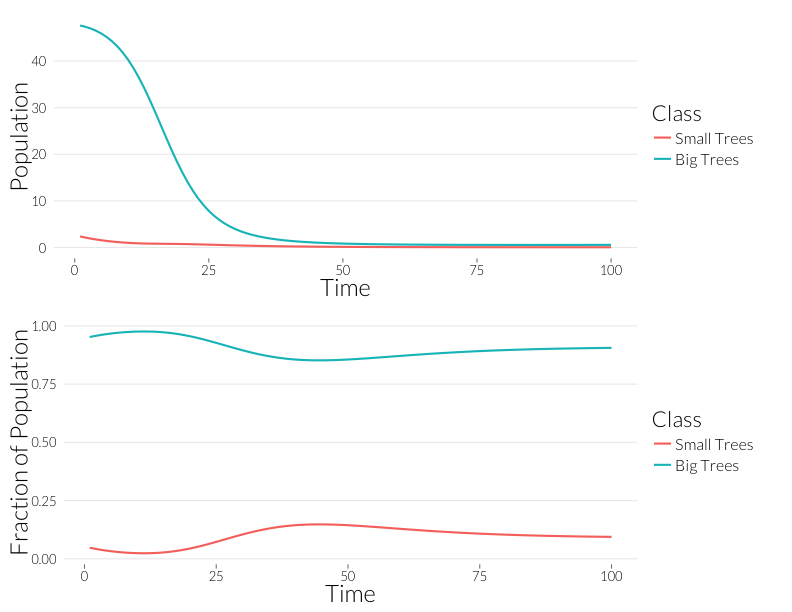
As in the \(SI\) model, the population drops, but the relative proportion of juvenile trees goes up. This occurs even though the mortality effect of one infection is the same on both classes. However, this could also be due to the fact that with fewer trees, density dependence has less of an effect on recruitment. Let’s look at the prevalance of disease, overall and per-tree:
p3 <- ggplot(subset(mdf, Class %in% c("PJ", "PA")),
             aes(x=Time, y=Population, col=Class)) +
      geom_line(lwd=1) + theme_nr + ylab("Number of Infections") + JAlab
p4 <- ggplot(subset(mdf, Class %in% c("nJ", "nA")),
             aes(x=Time, y=Population, col=Class)) +
      geom_line(lwd=1) + theme_nr + ylab("Infections per Individual") + JAlab
grid.arrange(p3, p4, nrow=2)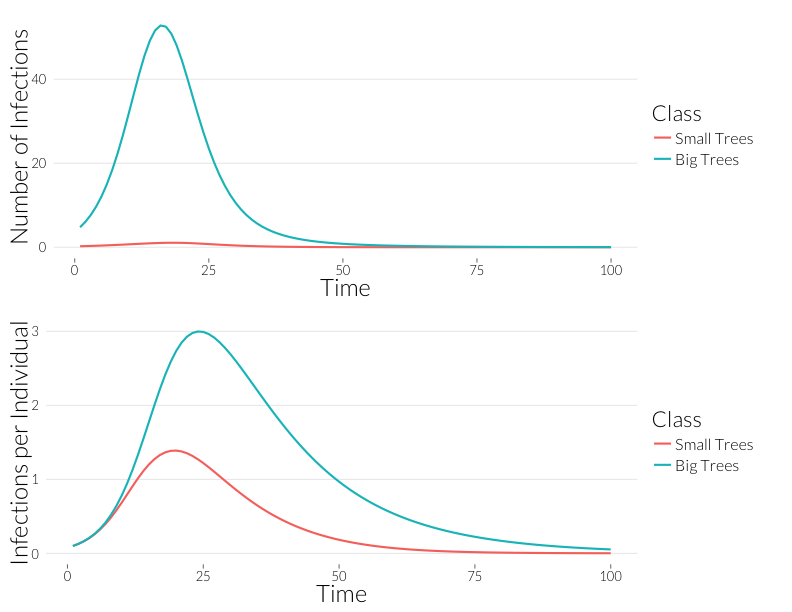
Infection is considerably greater in the adult trees than the juveniles over the course of the epidemic. Since, for the most part, observqtions of SOD don’t count the number of infections, it might be easier to look at this in terms of the number of trees infected. If we continue to assume a Poisson distribution of infections, we can calculate the fraction of infected trees as
\[\frac{I}{N} = 1 - e^{-\frac{P_N}{N}}\]
with \(N\) being a stand-in for \(J\) or \(A\).
ggplot(subset(mdf, Class %in% c("J.inf", "A.inf")),
       aes(x=Time, y=Population, col=Class)) +
geom_line(lwd=1) + theme_nr + ylab("Fraction infected") + JAlab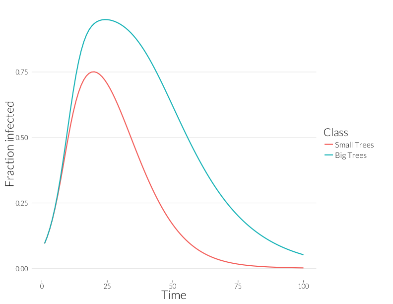
Note that these curves are somewhat closer to each other. Without observing multiple infections per tree, we might think distributions of disease in each size class are more similar than they really are.
So how does mortality differ between the classes? I calculate the “observed” mortality rate as the total mortality rate of only the diseased trees. This is:
\[d + \frac{\alpha P_N}{N (1 - \left( e^{- \frac{P_N}{N}}\right)}\]
The inverse of this value is “Years to infection”, which is the value shown in the right-hand panels of the figure from Cobb et al. (2012) above. Here I plot the “Years to mortality” that would be observed for trees in the model against the number of total infected trees in the population:
ggplot(subset(mdf, Class %in% c("J.yrs", "A.yrs") ),
       aes(x=Inf.dens, y=Population, col=Class)) +
  geom_point(cex=4) + theme_nr + xlab("Number of infected trees") +
  ylab("Years to death of infected individuals") + JAlab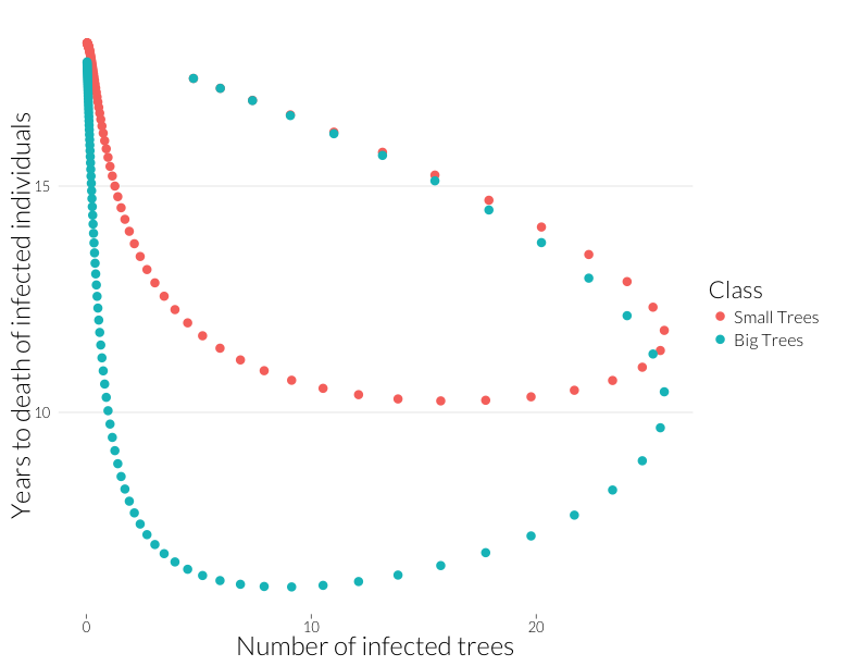
This plot is not quite equivalent to the lower-right panel in the figure from Cobb et al. (2012), because that shows a snapshot in time of many sites, while this shows the path of one site through time. Nonetheless, it shows that years-to-death has a negative relationship with the number of infected trees in this model, albeit a relationship that is state-dependent. That I can recreate this effect with this model suggests the multiple infection may drive this pattern.
Note that the mortality rate of both juveniles and adults start out the same (Years to death \(\approx\) 100), despite a higher adult population. I think ths means the difference of infection rates is not just due to a greater adult population, but due to the infections acquired by that class as more infected juveniles age into it.
The expression for the rate of infection of uninfected trees is:
\[\underbrace{1 - e^{-\left(\lambda (P_J + P_A) \frac{\overbrace{Ne^{(-P_N/N)}}^{\text{previously uninfected trees}}}{K}\right)}}_{\text{fraction newly infected}} \]
The inverse of this is “Years to Infection”, which I plot below against the number of infected trees.
ggplot(subset(mdf, Class %in% c("J.infyrs", "A.infyrs") ),
       aes(x=Inf.dens, y=Population, col=Class)) +
  geom_point(cex=4) + theme_nr + xlab("Number of infected trees") +
  ylab("Years to infection of uninfected individuals") + JAlab + ylim(0,200)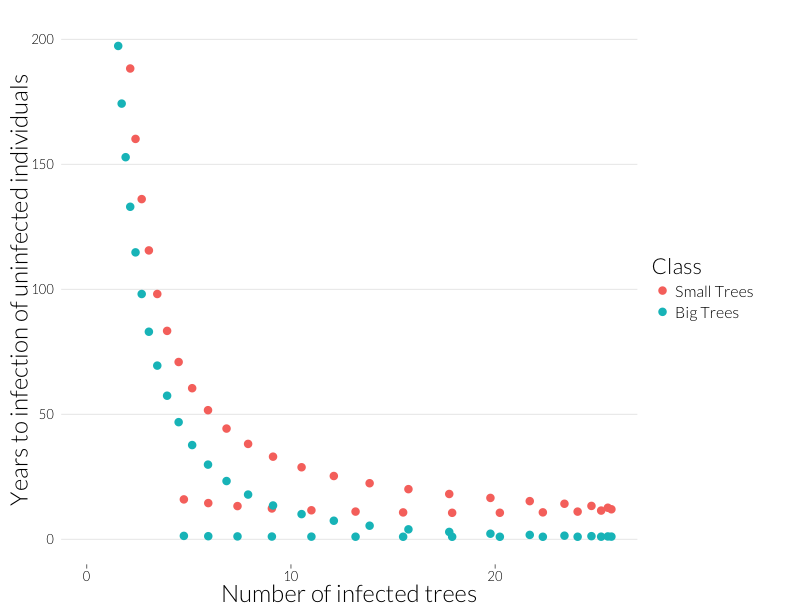
This is the rough equivalent to the bottom-left panel above from the Cobb et al. (2012). I’ve cut it off above 200 because years-to-infection quickly rise as the infection rate approaches zero. Neverthless, there’s a similar pattern to year-to-mortality, albeit shallower at the beginning and steeper at the end of the epidemic.
Next steps
This looks like a good start. This model is generating patterns observed in data on Sudden Oak Death in the wild, some explained and some unexplained. Some next steps:
- Examine the effect and robustness to overdisperal, when infections are distributed as a negative binomial. Ross Meentemeyer has data on the distribution of infections on Bay Laurel trees that may be useful in parameterizing this.
- Build in the multi-species case where there are reservoir/spreader species (Bay Laurel) and inert competitors (Redwood).
- Generalize to more size classes. Not strictly neccessary for prediction, but important for robustness.
References
Anderson, R. M., and R. M. May. 1978. Regulation and stability of host-parasite population interactions: I. Regulatory processes. The Journal of Animal Ecology 47:219–247.
Cobb, R. C., J. A. N. Filipe, R. K. Meentemeyer, C. A. Gilligan, and D. M. Rizzo. 2012. Ecosystem transformation by emerging infectious disease: loss of large tanoak from California forests. Journal of Ecology 100:712–722.